支持向量回归

References:

• [ML] 支持向量回归 | SVR | SVM
• SVR（Support Vactor Regression）支持向量回归机

【引入】

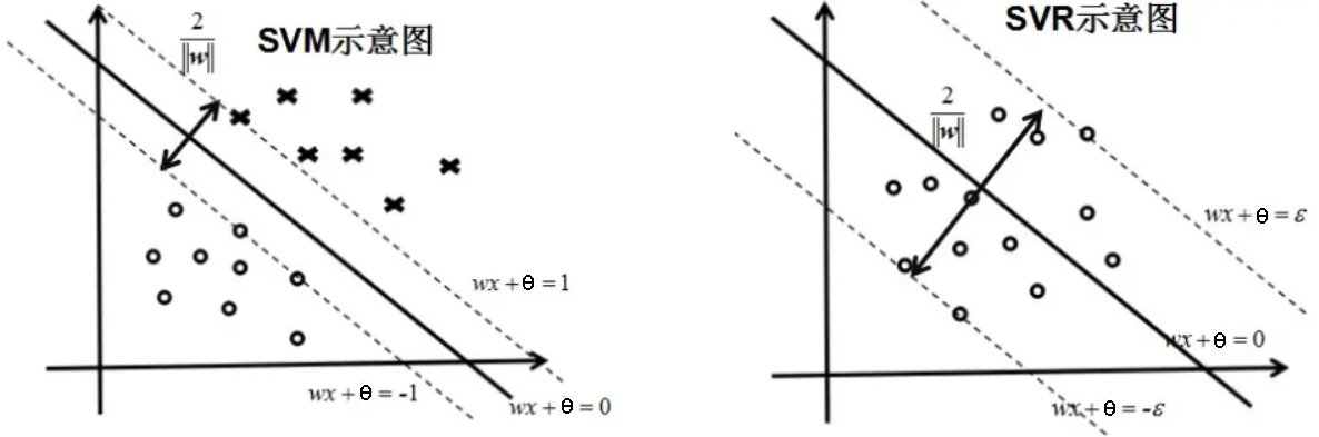
支持向量机是针对二分类问题提出的，其通过最大化间隔来找到一个分离超平面，使得绝大多数样本点位于两个决策边界的外侧

而支持向量回归（Support Vector Regression）是支持向量机的一种改进，用于解决回归问题，其同样是考虑最大化间隔，但是考虑的是两个决策边界之间的点，使尽可能多的样本点位于间隔内

换句话说，SVM 要使超平面到最近的样本点的间隔最大，SVR 则要使超平面到最远的样本点的间隔最小

【假设形式】

对于给定的容量为 $n$ 的训练集 $D=\{({\mathbf{x}}_{\mathbf{1}},y_1),({\mathbf{x}}_{\mathbf{2}},y_2),\dots ,({\mathbf{x}}_{\mathbf{n}},y_n)\}$，第 $i$ 组样本中的输入 ${\mathbf{x}}_{\mathbf{i}}$ 具有 $m$ 个特征值，即：${\mathbf{x}}_{\mathbf{i}}=(x_i^{(1)},x_i^{(2)},\dots ,x_i^{(m)})\in {\mathbb{R}}^m$，输出 $y_i\in \mathcal{Y}$，支持向量机学习到的模型为 $f(\mathbf{x})=\mathit{\omega }\cdot \mathbf{x}+\theta$，使得 $f({\mathbf{x}}_{\mathbf{i}})\simeq y_i$

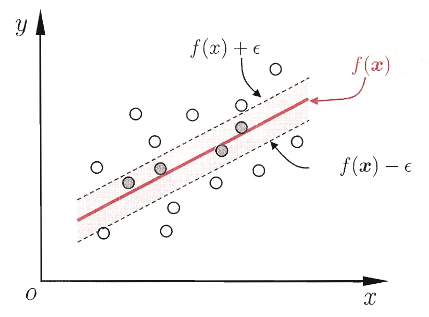
假设能容忍 $f({\mathbf{x}}_i)$ 与 $y_i$ 间最多有 $\epsilon$ 的偏差，即仅当 $f({\mathbf{x}}_i)$ 与 $y_i$ 之间差距的绝对值大于 $\epsilon$ 时才计算损失，这相当于以 $f(\mathbf{x})$ 为中心，构建了一个宽度为 $2\epsilon$ 的间隔带，若训练样本落于该间隔带，则认为预测正确

由此，可给出支持向量回归的优化问题：

$$\begin{array}{ccc}\underset{\mathit{\omega },\theta }{min}& & \frac{1}{2}||\mathit{\omega }|{|}_2^2\\ s.t.& & |y_i-(\mathit{\omega }\cdot {\mathbf{x}}_i+\theta )|\le \epsilon ,& & i=1,2,\cdots ,n\end{array}$$

其中，$\epsilon >0$ 是间隔带大小

通过求解最优化问题，可以得到超平面：

$$S:{\mathit{\omega }}^{\ast }\cdot \mathbf{x}+{\theta }^{\ast }=0$$

以及相应的回归函数：

$$f(\mathbf{x})={\mathit{\omega }}^{\ast }\cdot \mathbf{x}+{\theta }^{\ast }$$

【原始问题】

为每个样本点 $({\mathbf{x}}_i,y_i)$ 引入松弛变量 ${\xi }_i$ 和 $\widehat{{\xi }_i}$，即每个样本点分别到两个决策边界的距离

此时，支持向量回归的优化问题可写为：

$$\begin{array}{ccc}\underset{\mathit{\omega },\theta ,{\xi }_i,\widehat{{\xi }_i}}{min}& & \frac{1}{2}||\mathit{\omega }|{|}_2^2+C\sum _{i=1}^n({\xi }_i+\widehat{{\xi }_i})\\ s.t.& & y_i-(\mathit{\omega }\cdot {\mathbf{x}}_i+\theta )\le \epsilon +{\xi }_i\\ & & (\mathit{\omega }\cdot {\mathbf{x}}_i+\theta )-y_i\le \epsilon +\widehat{{\xi }_i}\\ & & {\xi }_i\ge 0\\ & & \widehat{{\xi }_i}\ge 0,& & i=1,2,\cdots ,n\end{array}$$

即为支持向量回归的原始问题，其中，$C$ 为正则化常数

可以发现，支持向量回归只对间隔外的样本进行惩罚，当样本点位于间隔内，不计算其损失

【对偶问题】

对偶问题的转化

为求解支持向量回归的原始问题：

$$\begin{array}{ccc}\underset{\mathit{\omega },\theta ,{\xi }_i,\widehat{{\xi }_i}}{min}& & \frac{1}{2}||\mathit{\omega }|{|}_2^2+C\sum _{i=1}^n({\xi }_i+\widehat{{\xi }_i})\\ s.t.& & y_i-(\mathit{\omega }\cdot {\mathbf{x}}_i+\theta )\le \epsilon +{\xi }_i\\ & & (\mathit{\omega }\cdot {\mathbf{x}}_i+\theta )-y_i\le \epsilon +\widehat{{\xi }_i}\\ & & {\xi }_i\ge 0\\ & & \widehat{{\xi }_i}\ge 0,& & i=1,2,\cdots ,n\end{array}$$

应用拉格朗日对偶性，通过求解对偶问题来得到原始问题的最优解

首先，构建拉格朗日函数，即为每个不等式约束引入拉格朗日乘子 ${\lambda }_i\ge 0$、$\widehat{{\lambda }_i}\ge 0$、${\mu }_i\ge 0$、$\widehat{{\mu }_i}\ge 0$，即：

$$\begin{array}{rl}L(\mathit{\omega },\theta ,\mathit{\xi },\hat{\mathit{\xi }},\mathit{\lambda },\hat{\mathit{\lambda }},\mathit{\mu },\hat{\mathit{\mu }})=& \frac{1}{2}||\mathit{\omega }|{|}_2^2+C\sum _{i=1}^n({\xi }_i+\widehat{{\xi }_i})+\sum _{i=1}^n{\lambda }_i(y_i-(\mathit{\omega }\cdot {\mathbf{x}}_i+\theta )-\epsilon -{\xi }_i)\\ & +\sum _{i=1}^n\widehat{{\lambda }_i}((\mathit{\omega }\cdot {\mathbf{x}}_i+\theta )-y_i-\epsilon -\widehat{{\xi }_i})-\sum _{i=1}^n{\mu }_i{\xi }_i-\sum _{i=1}^n\widehat{u_i}\widehat{{\xi }_i}\end{array}$$

其中，$\mathit{\lambda }=({\lambda }_1,{\lambda }_2,\dots ,{\lambda }_n{)}^T$、$\hat{\mathit{\lambda }}=(\widehat{{\lambda }_1},\widehat{{\lambda }_2},\dots ,\widehat{{\lambda }_n}{)}^T$、$\mathit{\mu }=({\mu }_1,{\mu }_2,\dots ,{\mu }_n{)}^T$、$\hat{\mathit{\mu }}=(\widehat{{\mu }_1},\widehat{{\mu }_2},\dots ,\widehat{{\mu }_n}{)}^T$ 为拉格朗日乘子向量

此时，根据拉格朗日对偶性，原始问题的对偶问题就变为极大极小问题，即：

$$\underset{\mathit{\lambda },\hat{\mathit{\lambda }},\mathit{\mu },\hat{\mathit{\mu }}}{max}\underset{\mathit{\omega },\theta ,\mathit{\xi },\hat{\mathit{\xi }}}{min}L(\mathit{\omega },\theta ,\mathit{\xi },\hat{\mathit{\xi }},\mathit{\lambda },\hat{\mathit{\lambda }},\mathit{\mu },\hat{\mathit{\mu }})$$

因此，为了得到对偶问题的解，就要先求拉格朗日函数 $L(\mathit{\omega },\theta ,\mathit{\xi },\hat{\mathit{\xi }},\mathit{\lambda },\hat{\mathit{\lambda }},\mathit{\mu },\hat{\mathit{\mu }})$ 对 $\mathit{\omega }$、$\theta$、$\mathit{\xi }$、$\hat{\mathit{\xi }}$ 的极小，再求对 $\mathit{\lambda }$、$\hat{\mathit{\lambda }}$、$\mathit{\mu }$、$\hat{\mathit{\mu }}$ 的极大

对偶问题中的极小问题

对于对偶问题中的极小问题：

$$\underset{\mathit{\omega },\theta ,\mathit{\xi },\hat{\mathit{\xi }}}{min}L(\mathit{\omega },\theta ,\mathit{\xi },\hat{\mathit{\xi }},\mathit{\lambda },\hat{\mathit{\lambda }},\mathit{\mu },\hat{\mathit{\mu }})$$

令拉格朗日函数 $L(\mathit{\omega },\theta ,\mathit{\xi },\hat{\mathit{\xi }},\mathit{\lambda },\hat{\mathit{\lambda }},\mathit{\mu },\hat{\mathit{\mu }})$ 分别对 $\mathit{\omega }$、$\theta$、$\mathit{\xi }$、$\hat{\mathit{\xi }}$ 求偏导，并令其等于 $0$，即：

$$\begin{array}{rl}{▽}_{\mathit{\omega }}L(\mathit{\omega },\theta ,\mathit{\xi },\hat{\mathit{\xi }},\mathit{\lambda },\hat{\mathit{\lambda }},\mathit{\mu },\hat{\mathit{\mu }})& =\mathit{\omega }-\sum _{i=1}^n({\lambda }_i-\widehat{{\lambda }_i}){\mathbf{x}}_i=0\\ {▽}_{\mathit{\theta }}L(\mathit{\omega },\theta ,\mathit{\xi },\hat{\mathit{\xi }},\mathit{\lambda },\hat{\mathit{\lambda }},\mathit{\mu },\hat{\mathit{\mu }})& =\sum _{i=1}^n({\lambda }_i-\widehat{{\lambda }_i})=0\\ {▽}_{{\mathit{\xi }}_{\mathit{i}}}L(\mathit{\omega },\theta ,\mathit{\xi },\hat{\mathit{\xi }},\mathit{\lambda },\hat{\mathit{\lambda }},\mathit{\mu },\hat{\mathit{\mu }})& =C-{\lambda }_i-{\mu }_i=0\\ {▽}_{\widehat{{\mathit{\xi }}_{\mathit{i}}}}L(\mathit{\omega },\theta ,\mathit{\xi },\hat{\mathit{\xi }},\mathit{\lambda },\hat{\mathit{\lambda }},\mathit{\mu },\hat{\mathit{\mu }})& =C-\widehat{{\lambda }_i}-\widehat{{\mu }_i}=0\end{array}$$

可得：

$$\begin{array}{c}\mathit{\omega }=\sum _{i=1}^n({\lambda }_i-\widehat{{\lambda }_i}){\mathbf{x}}_i\\ \sum _{i=1}^n({\lambda }_i-\widehat{{\lambda }_i})=0\\ C={\lambda }_i+{\mu }_i\\ C=\widehat{{\lambda }_i}+\widehat{{\mu }_i}\end{array}$$

将上式带回拉格朗日函数 $L(\mathit{\omega },\theta ,\mathit{\xi },\hat{\mathit{\xi }},\mathit{\lambda },\hat{\mathit{\lambda }},\mathit{\mu },\hat{\mathit{\mu }})$ 中，有：

$$\begin{array}{rl}& L(\mathit{\omega },\theta ,\mathit{\xi },\hat{\mathit{\xi }},\mathit{\lambda },\hat{\mathit{\lambda }},\mathit{\mu },\hat{\mathit{\mu }})\\ =& \frac{1}{2}||\mathit{\omega }|{|}_2^2+C\sum _{i=1}^n({\xi }_i+\widehat{{\xi }_i})+\sum _{i=1}^n{\lambda }_i(y_i-(\mathit{\omega }\cdot {\mathbf{x}}_i+\theta )-\epsilon -{\xi }_i)\\ & +\sum _{i=1}^n\widehat{{\lambda }_i}((\mathit{\omega }\cdot {\mathbf{x}}_i+\theta )-y_i-\epsilon -\widehat{{\xi }_i})-\sum _{i=1}^n{\mu }_i{\xi }_i-\sum _{i=1}^n\widehat{u_i}\widehat{{\xi }_i}\\ =& \frac{1}{2}\sum _{i=1}^n\sum _{j=1}^m({\lambda }_i-\widehat{{\lambda }_i})({\lambda }_j-\widehat{{\lambda }_j}){\mathbf{x}}_i\cdot {\mathbf{x}}_j+\sum _{i=1}^n(C{\xi }_i+C\widehat{{\xi }_i})\\ & +\sum _{i=1}^n{\lambda }_i{y}_i-\sum _{i=1}^n{\lambda }_i\mathit{\omega }\cdot {\mathbf{x}}_i-\theta \sum _{i=1}^n{\lambda }_i-\epsilon \sum _{i=1}^n{\lambda }_i-\sum _{i=1}^n{\lambda }_i{\xi }_i\\ & -\sum _{i=1}^n\widehat{{\lambda }_i}{y}_i+\sum _{i=1}^n\widehat{{\lambda }_i}\mathit{\omega }\cdot {\mathbf{x}}_i+\theta \sum _{i=1}^n\widehat{{\lambda }_i}-\epsilon \sum _{i=1}^n\widehat{{\lambda }_i}-\sum _{i=1}^n\widehat{{\lambda }_i}\widehat{{\xi }_i}\\ & -\sum _{i=1}^n{\mu }_i{\xi }_i-\sum _{i=1}^n\widehat{u_i}\widehat{{\xi }_i}\\ =& \frac{1}{2}\sum _{i=1}^n\sum _{j=1}^m({\lambda }_i-\widehat{{\lambda }_i})({\lambda }_j-\widehat{{\lambda }_j}){\mathbf{x}}_i\cdot {\mathbf{x}}_j-\sum _{i=1}^n({\lambda }_i-\widehat{{\lambda }_i})\mathit{\omega }\cdot {\mathbf{x}}_i\\ & +\sum _{i=1}^n({\lambda }_i-\widehat{{\lambda }_i})y_i-\theta \sum _{i=1}^n({\lambda }_i-\widehat{{\lambda }_i})-\epsilon \sum _{i=1}^n({\lambda }_i+\widehat{{\lambda }_i})\\ & +\sum _{i=1}^n(({\lambda }_i+{\mu }_i){\xi }_i+(\widehat{{\lambda }_i}+\widehat{{\mu }_i})\widehat{{\xi }_i})-\sum _{i=1}^n({\mu }_i{\xi }_i+{\lambda }_i{\xi }_i+\widehat{{\lambda }_i}\widehat{{\xi }_i}+\widehat{u_i}\widehat{{\xi }_i})\\ =& -\frac{1}{2}\sum _{i=1}^n\sum _{j=1}^m({\lambda }_i-\widehat{{\lambda }_i})({\lambda }_j-\widehat{{\lambda }_j}){\mathbf{x}}_i\cdot {\mathbf{x}}_j+\sum _{i=1}^n({\lambda }_i-\widehat{{\lambda }_i})y_i-\epsilon \sum _{i=1}^n({\lambda }_i+\widehat{{\lambda }_i})\end{array}$$

故有：

$$\begin{array}{rl}\underset{\mathit{\omega },\theta ,\mathit{\xi },\hat{\mathit{\xi }}}{min}L(\mathit{\omega },\theta ,\mathit{\xi },\hat{\mathit{\xi }},\mathit{\lambda },\hat{\mathit{\lambda }},\mathit{\mu },\hat{\mathit{\mu }})=& -\frac{1}{2}\sum _{i=1}^n\sum _{j=1}^m({\lambda }_i-\widehat{{\lambda }_i})({\lambda }_j-\widehat{{\lambda }_j}){\mathbf{x}}_i\cdot {\mathbf{x}}_j\\ & +\sum _{i=1}^n({\lambda }_i-\widehat{{\lambda }_i})y_i-\epsilon \sum _{i=1}^n({\lambda }_i+\widehat{{\lambda }_i})\end{array}$$

对偶问题中的极大问题

对于对偶问题中的极大问题：

$$\underset{\mathit{\lambda },\hat{\mathit{\lambda }},\mathit{\mu },\hat{\mathit{\mu }}}{max}\underset{\mathit{\omega },\theta ,\mathit{\xi },\hat{\mathit{\xi }}}{min}L(\mathit{\omega },\theta ,\mathit{\xi },\hat{\mathit{\xi }},\mathit{\lambda },\hat{\mathit{\lambda }},\mathit{\mu },\hat{\mathit{\mu }})$$

即为对偶问题，有：

$$\begin{array}{ccc}\underset{\mathit{\lambda },\hat{\mathit{\lambda }}}{max}& & -\frac{1}{2}\sum _{i=1}^n\sum _{j=1}^m({\lambda }_i-\widehat{{\lambda }_i})({\lambda }_j-\widehat{{\lambda }_j}){\mathbf{x}}_i\cdot {\mathbf{x}}_j+\sum _{i=1}^n({\lambda }_i-\widehat{{\lambda }_i})y_i-\epsilon \sum _{i=1}^n({\lambda }_i+\widehat{{\lambda }_i})\\ s.t.& & \sum _{i=1}^n({\lambda }_i-\widehat{{\lambda }_i})=0\\ & & 0\le {\lambda }_i,\widehat{{\lambda }_i}\le C,i=1,2,\cdots ,n\end{array}$$

假设上述的对偶问题对 $\mathit{\lambda }$、$\hat{\mathit{\lambda }}$、$\mathit{\xi }$、$\hat{\mathit{\xi }}$ 的一个解为 ${\mathit{\lambda }}^{\ast }=({\lambda }_1^{\ast },{\lambda }_2^{\ast },\cdots ,{\lambda }_n^{\ast }{)}^T$， ${\hat{\mathit{\lambda }}}^{\ast }=({\widehat{{\lambda }_1}}^{\ast },{\widehat{{\lambda }_2}}^{\ast },\cdots ,{\widehat{{\lambda }_n}}^{\ast }{)}^T$、${\mathit{\xi }}^{\ast }=({\xi }_1^{\ast },{\xi }_2^{\ast },\cdots ,{\xi }_n^{\ast }{)}^T$， ${\hat{\mathit{\xi }}}^{\ast }=({\widehat{{\xi }_1}}^{\ast },{\widehat{{\xi }_2}}^{\ast },\cdots ,{\widehat{{\xi }_n}}^{\ast }{)}^T$、

可以发现，对偶问题满足 KKT 条件，即：

$$\begin{array}{c}{\lambda }_i^{\ast }(\mathit{\omega }\cdot \mathbf{x}+\theta )-y_i-\epsilon -{\xi }_i^{\ast })=0\\ \widehat{{\lambda }_i^{\ast }}(\mathit{\omega }\cdot \mathbf{x}+\theta )-y_i-\epsilon -\widehat{{\xi }_i^{\ast }})=0\\ {\lambda }_i^{\ast }\widehat{{\lambda }_i^{\ast }}=0\\ {\xi }_i^{\ast }\widehat{{\xi }_i^{\ast }}=0\\ (C-{\lambda }_i^{\ast }){\xi }_i^{\ast }=0\\ (C-\widehat{{\lambda }_i^{\ast }})\widehat{{\xi }_i^{\ast }}=0\end{array}$$

故而有：

$${\mathit{\omega }}^{\ast }=\sum _{i=1}^n({\lambda }_i-\widehat{{\lambda }_i}){\mathbf{x}}_i$$

可以看出，当且仅当 $(\mathit{\omega }\cdot \mathbf{x}+\theta )-y_i-\epsilon -{\xi }_i^{\ast }=0$ 时，${\lambda }_i^{\ast }$ 可取非零值，当且仅当 $(\mathit{\omega }\cdot \mathbf{x}+\theta )-y_i-\epsilon -{\widehat{{\xi }_i}}^{\ast }=0$ 时，${\widehat{{\lambda }_i}}^{\ast }$ 可取非零值，换言之，仅当样本 $({\mathbf{x}}_i,y_i)$ 不落于 $\epsilon$ 间隔带时，相应的 ${\lambda }_i$ 和 $\widehat{{\lambda }_i}$ 才可取非零值

此外，约束 $(\mathit{\omega }\cdot \mathbf{x}+\theta )-y_i-\epsilon -{\xi }_i^{\ast }=0$ 和 $(\mathit{\omega }\cdot \mathbf{x}+\theta )-y_i-\epsilon -{\widehat{{\xi }_i}}^{\ast }=0$ 不能同时成立，否则有 ${\xi }_i^{\ast }=\widehat{{\xi }_i^{\ast }}=\epsilon$，因此 ${\lambda }_i$ 和 $\widehat{{\lambda }_i}$ 中至少有一个为零，即 ${\lambda }_i\widehat{{\lambda }_i}$

而对于每个样本 $({\mathbf{x}}_i,y_i)$，都有 $(C-{\lambda }_i^{\ast }){\xi }_i^{\ast }=0$ 且 $(\mathit{\omega }\cdot \mathbf{x}+\theta )-y_i-\epsilon -{\xi }_i^{\ast }=0$，于是在得到 ${\lambda }_i^{\ast }$ 后，若存在 $0<{\lambda }_i^{\ast }<C$，那么必有 ${\xi }_i^{\ast }=0$，进而对此 $i$ 有：

$${\theta }^{\ast }=y_i+\epsilon -\sum _{j=1}^n({\lambda }_i^{\ast }-\widehat{{\lambda }_i^{\ast }}){\mathbf{x}}_j\cdot {\mathbf{x}}_i$$

理论上来说，可以任意选取满足 $0<{\lambda }_i^{\ast }<C$ 的样本，通过上式得到 $\theta$，但在实际应用中，常选取所有的满足 $0<{\lambda }_i^{\ast }<C$ 的样本，求取相应的 $\theta$ 后求其平均值 $\bar{\theta }$

故而，当 ${\lambda }_i-\widehat{{\lambda }_i}\ne 0$ 时，有回归函数：

$$f(\mathbf{x})=\sum _{i=1}^n({\lambda }_i-\widehat{{\lambda }_i})({\mathbf{x}}_i\cdot \mathbf{x})+\bar{\theta }$$

【非线性支持向量回归】

对于回归函数：

$$f(\mathbf{x})=\sum _{i=1}^n({\lambda }_i-\widehat{{\lambda }_i})({\mathbf{x}}_i\cdot \mathbf{x})+\bar{\theta }$$

若考虑到非线性问题，可以参照非线性支持向量机的思路，使用核方法进行特征构建，引入核函数即可，故非线性 SVR 可表示为：

$$f(\mathbf{x})=\sum _{i=1}^n({\lambda }_i-\widehat{{\lambda }_i})K({\mathbf{x}}_i,\mathbf{x})+\bar{\theta }$$

关于核函数，详见：特征构建与核方法

【sklearn 实现】

线性支持向量回归

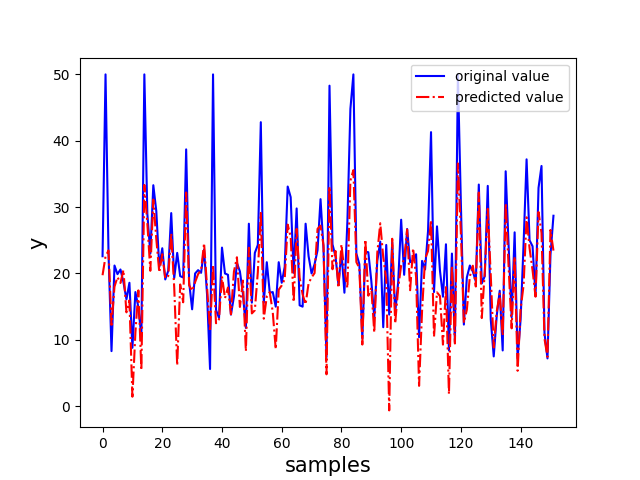
以 sklearn 中的波士顿房价数据集为例，实现线性支持向量回归

import numpy as np
import pandas as pd
import matplotlib.pyplot as plt
from sklearn.datasets import load_boston
from sklearn.model_selection import train_test_split
from sklearn.svm import LinearSVR
from sklearn.metrics import mean_squared_error
from sklearn.metrics import mean_squared_error
from sklearn.metrics import mean_absolute_error
from sklearn.metrics import r2_score

# 特征提取
def deal_data():
    boston = load_boston()  # sklearn的波士顿房价数据集
    df = pd.DataFrame(boston.data, columns=boston.feature_names)
    df['result'] = boston.target
    data = np.array(df)
    return data[:, :-1], data[:, -1]

# 模型训练
def train_model(features, labels):  
    # 建立线性支持向量回归模型
    model = LinearSVR(random_state=0, tol=1e-05)
    
    # 训练
    model.fit(features, labels)
    return model

# 模型评估
def estimate_model(y_true, y_pred):
    MSE = mean_squared_error(y_true, y_pred)
    RMSE = np.sqrt(MSE)
    MAE = mean_absolute_error(y_true, y_pred)
    R2 = r2_score(y_true, y_pred)
    indicators = {"MSE": MSE, "RMSE":RMSE, "MAE":MAE, "R2":R2}
    return indicators

# 可视化
def visualization(y_true, y_pred, model):
    # 绘图
    plt.plot(range(y_true.shape[0]), y_true, "b-") 
    plt.plot(range(y_true.shape[0]), y_pred, "r-.")
    plt.legend(["original value", "predicted value"])
    plt.xlabel("samples", fontsize="15")
    plt.ylabel("y", fontsize="15")
    
    plt.show()

if __name__ == "__main__":
    # 特征提取
    x, y = deal_data()
    
    # 简单交叉验证
    x_train, x_test, y_train, y_test = train_test_split(x, y, test_size=0.3, random_state=0)
    
    # 模型训练
    model = train_model(x_train, y_train)
    
    # 预测结果
    y_pred = model.predict(x_test) # predict()输入输出均为二维
    print("y test:", y_test[:10]) # 测试集y值
    print("y pred:", y_pred[:10]) # 预测y值
    
    # 模型评估
    indicators = estimate_model(y_test, y_pred)
    print("MSE:", indicators["MSE"])
    print("RMSE:", indicators["RMSE"])
    print("MAE:", indicators["MAE"])
    print("R2:", indicators["R2"])
    
    # 可视化
    visualization(y_test, y_pred, model)

非线性支持向量回归

以 sklearn 中的波士顿房价数据集为例，实现线性支持向量回归

import numpy as np
import pandas as pd
import matplotlib.pyplot as plt
from sklearn.datasets import load_boston
from sklearn.model_selection import train_test_split
from sklearn.svm import SVR
from sklearn.metrics import mean_squared_error
from sklearn.metrics import mean_squared_error
from sklearn.metrics import mean_absolute_error
from sklearn.metrics import r2_score

# 特征提取
def deal_data():
    boston = load_boston()  # sklearn的波士顿房价数据集
    df = pd.DataFrame(boston.data, columns=boston.feature_names)
    df['result'] = boston.target
    data = np.array(df)
    return data[:, :-1], data[:, -1]

# 模型训练
def train_model(features, labels):  
    # 建立非线性SVR模型
    # kernel可选：
    #  - linear：线性核函数，与LinearSVR效果一致，但速度较慢
    #  - poly：多项式核函数，gamma为多项式的系数，degree为多项式的次数，coef0为多项式截距
    #  - rbf：高斯核函数，gamma为1/2σ
    #  - sigmoid：sigmoid核函数，coef0为多项式截距
    model = SVR(kernel='rbf', degree=3, C=1.0, epsilon=0.2)
    
    # 训练
    model.fit(features, labels)
    return model

# 模型评估
def estimate_model(y_true, y_pred):
    MSE = mean_squared_error(y_true, y_pred)
    RMSE = np.sqrt(MSE)
    MAE = mean_absolute_error(y_true, y_pred)
    R2 = r2_score(y_true, y_pred)
    indicators = {"MSE": MSE, "RMSE":RMSE, "MAE":MAE, "R2":R2}
    return indicators

# 可视化
def visualization(y_true, y_pred, model):
    # 绘图
    plt.plot(range(y_true.shape[0]), y_true, "b-") 
    plt.plot(range(y_true.shape[0]), y_pred, "r-.")
    plt.legend(["original value", "predicted value"])
    plt.xlabel("samples", fontsize="15")
    plt.ylabel("y", fontsize="15")
    
    plt.show()

if __name__ == "__main__":
    # 特征提取
    x, y = deal_data()
    
    # 简单交叉验证
    x_train, x_test, y_train, y_test = train_test_split(x, y, test_size=0.3,random_state=0)
    
    # 模型训练
    model = train_model(x_train, y_train)
    
    # 预测结果
    y_pred = model.predict(x_test) # predict()输入输出均为二维
    print("y test:", y_test[:10]) # 测试集y值
    print("y pred:", y_pred[:10]) # 预测y值
    
    # 模型评估
    indicators = estimate_model(y_test, y_pred)
    print("MSE:", indicators["MSE"])
    print("RMSE:", indicators["RMSE"])
    print("MAE:", indicators["MAE"])
    print("R2:", indicators["R2"])
    
    # 可视化
    visualization(y_test, y_pred, model)