References:
【引入】
软隔支持向量机是用来解决训练集近似线性可分情况的二分类模型,但其无法处理线性不可分的情况
为解决该问题,在软间隔支持向量机的基础上引入了核方法,通过一个非线性变换将输入空间对应于一个特征空间,从而使得在输入空间中的超曲面模型对应于特征空间中的超平面模型
这样,分类问题的学习任务通过在特征空间中求解软间隔支持向量机即可完成

【假设形式】
非线性支持向量机(Non-linear Support Vector Machine)是将软间隔支持向量机的输入空间通过映射函数 $\phi(\mathbf{x})$ 变换到一个新的特征空间,并将输入空间的内积 $\mathbf{x}_i\cdot\mathbf{x}_j$ 变换为特征空间中的内积 $\phi(\mathbf{x}_i)\cdot\phi(\mathbf{x}_j)$,在新的特征空间中从训练样本中学习软间隔支持向量机
对于容量为 $n$ 的线性不可分的训练集 $D=\{(\mathbf{x}_1,y_1),(\mathbf{x}_2,y_2),…,(\mathbf{x}_n,y_n)\}$,第 $i$ 组样本中的输入 $\mathbf{x}_i$ 具有 $m$ 个特征值,即:$\mathbf{x}_i=(x_i^{(1)},x_i^{(2)},…,x_i^{(m)})\in \mathbb{R}^m$,输出 $y_i\in\mathcal{Y}=\{+1,-1\}$
软间隔支持向量机学习算法的对偶问题:
目标函数只涉及到输入实例与输入实例间的内积,将内积 $\mathbf{x}_i\cdot\mathbf{x}_j$ 用正定核函数 $K(\mathbf{x}_i,\mathbf{x}_j)=\phi(\mathbf{x}_i)\cdot\phi(\mathbf{x}_j)$ 来代替,此时对偶问题的目标函数为:
同样,分类决策函数中的内积也用核函数来代替:
这样一来,当映射函数 $\phi(\mathbf{x})$ 是非线性函数时,学习到的含有核函数的支持向量机就是非线性分类模型,即非线性支持向量机
关于核函数,详见:特征构建与核方法
【核技巧】
对于核方法来说,直接计算核函数 $K(\mathbf{x},\mathbf{z})$ 比较容易,而通过映射函数 $\phi(\mathbf{x})$ 和 $\phi(\mathbf{z})$ 计算 $K(\mathbf{x},\mathbf{z})$ 较为复杂
核技巧(Kernel Trick)是一种加速核方法的计算技巧,其在学习和预测中只显式的定义核函数 $K(\mathbf{x},\mathbf{z})$,不显式的定义 $\phi(\mathbf{x})$ 和 $\phi(\mathbf{z})$ ,从而避开分别计算 $\phi(\mathbf{x})$ 和 $\phi(\mathbf{z})$
利用核技巧,在核函数 $K(\mathbf{x},\mathbf{z})$ 给定的情况下,可以将线性分类的学习方法应用到非线性分类问题中,对于支持向量机来说,可以将软间隔支持向量机扩展到非线性支持向量机
在实际应用中,往往依赖于领域知识来直接选择核函数,而核函数选择的有效性需要通过实验验证
【学习算法】
下面给出非线性支持向量机的学习算法:
输入:容量为 $n$ 的线性不可分的训练集 $D=\{(\mathbf{x}_1,y_1),(\mathbf{x}_2,y_2),…,(\mathbf{x}_n,y_n)\}$,第 $i$ 组样本中的输入 $\mathbf{x}_i$ 具有 $m$ 个特征值,即:$\mathbf{x}_i=(x_i^{(1)},x_i^{(2)},…,x_i^{(m)})\in \mathbb{R}^m$,输出 $y_i\in\mathcal{Y}=\{+1,-1\}$
输出:分类决策函数
算法步骤:
Step1:选择适当的核函数 $K(\mathbf{x},\mathbf{z})$ 惩罚系数 $C>0$,构造并求解如下约束最优化问题(原始问题的对偶问题)
求得最优解 $\boldsymbol{\lambda}^* = (\lambda_1^*,\lambda_2^*,\cdots,\lambda_n^*)^T$
Step2:根据最优解 $\boldsymbol{\lambda}^*$,选择一个正分量 $0<\lambda_j^*<C$,计算截距 $\theta^*$:
Step3:根据最优解 $\boldsymbol{\lambda}^*$ 和 $\theta^*$,构建分类决策函数
对于 Step1 中的约束最优化问题,当 $K(\mathbf{x},\mathbf{z})$ 是正定核函数时,其是一个凸二次规划问题,可以使用 SMO 算法求解,关于 SMO 算法,详见:序列最小最优化算法 SMO
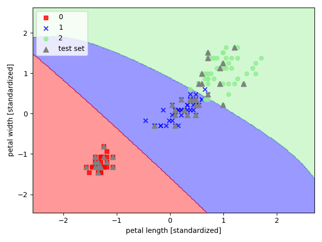
【sklearn 实现】
以 sklearn 中的鸢尾花数据集为例,选取其后两个特征来实现非线性支持向量机
1 | import pandas as pd |