一元线性回归

【假设形式】

在回归分析中，只有一个自变量和因变量，且因变量和自变量之间是线性关系，一般称为一元线性回归（Unary Linear Regression）

通过线性回归算法，会得到很多的线性回归模型，但是不同的模型对于数据的拟合（描述能力）是不一样的，我们的目的是找到一个能够最精确描述数据之间关系的线性回归模型

其假设形式如下：

对于给定的容量为 $n$ 的样本集 $D=\{(x_1,y_1),(x_2,y_2),…,(x_n,y_n)\}$，第 $i$ 组样本中的输入为 $x_i$，输出为 $y_i$

假设一元线性回归学习到的模型是 $f(x_i;\theta_0,\theta_1)=\theta_0+\theta_1 x_i$，使得 $f(x_i;\theta_0,\theta_1)\simeq y_i$

若要使预测更为精确，那么预测就要以现有的数据为根基，尽量的贴合现有数据，使得预测值与真实值的差距尽量小

这就需要一个损失函数 $J(\theta_0,\theta_1)$ 来作为衡量预测结果的指标，对于损失函数最小化时的 $\theta_0$ 与 $\theta_1$，通常使用最小二乘法或以梯度下降法为代表的迭代法来求解

无论使用何种方法，最终的目标，都是要令这个损失函数的值最小化，即

$$(\theta_0^*,\theta_1^*) = \arg \min \limits_{(\theta_0,\theta_1)} \:J(\theta_0,\theta_1)$$

【梯度下降法求解】

对于给定的容量为 $n$ 的样本集 $D=\{(x_1,y_1),(x_2,y_2),…,(x_n,y_n)\}$，第 $i$ 组样本中的输入为 $x_i$，输出为 $y_i$

设习得的模型的假设函数为：

$$f(x_i;\theta_0,\theta_1)=\theta_0+\theta_1 x_i$$

令损失函数为：

$$J(\theta_0,\theta_1) = \frac{1}{2n} \sum\limits_{i=1}^{n} (f(x_i;\theta_0,\theta_1) - y_i )^2$$

之所以要乘以 $\frac{1}{2}$，是因为在求导后会带来 $\times 2$，不利于表达与计算，当乘以 $\frac{1}{2}$ 后，求导带来的 $\times 2$ 就与 $\frac{1}{2}$ 抵消，从而简化计算

目标是通过最小化代价函数 $J(\theta_0,\theta_1)$ 来在参数空间 $\Theta$ 中找到合适的 $\theta_0,\theta_1$ 参数，即：

$$(\theta_0^*,\theta_1^*) = \arg \min \limits_{(\theta_0,\theta_1)} \:J(\theta_0,\theta_1)$$

在最小化代价函数 $J(\theta_0,\theta_1)$ 时，其核心是损失函数对应的梯度函数，使用梯度下降法，即将下列公式重复直到收敛为止：

$$\boldsymbol{\theta_{k+1}} = \boldsymbol{\theta_k} - \alpha \frac{\partial}{\partial \boldsymbol{\theta_k}}J(\boldsymbol{\theta_k})$$

即：

$$\left\{\begin{array}{rl} \theta_0 & = & \theta_0 - \alpha \sum\limits_{i=1}^n (f(x_i;\theta_0,\theta_1) - y_i) \\ \theta_1 & = & \theta_1 - \alpha \sum\limits_{i=1}^n (f(x_i;\theta_0,\theta_1) - y_i)\cdot x_i \end{array} \right.$$

关于批量梯度下降法的具体介绍，详见：梯度下降法

【最小二乘法求解】

当使用最小二乘法来求解时，一般选用残差平方和 RSS 作为损失函数，即：

$$\begin{align} J(\theta_0,\theta_1) & = \sum_{i=1}^n(f(x_i;\theta_0,\theta_1)-y_i)^2 \notag \\ & = \sum_{i=1}^n( \theta_0 + \theta_1 x_i-y_i)^2 \notag \end{align}$$

目标是通过最小化代价函数 $J(\theta_0,\theta_1)$ 来在参数空间 $\Theta$ 中找到合适的 $\theta_0,\theta_1$ 参数，即：

$$(\theta_0^*,\theta_1^*) = \arg \min \limits_{(\theta_0,\theta_1)} \:J(\theta_0,\theta_1)$$

在最小化代价函数 $J(\theta_0,\theta_1)$ 时，其核心是损失函数对应的梯度函数，分别对 $J(\theta_0,\theta_1)$ 分别对 $\theta_0$、$\theta_1$ 进行求导，有：

$$\left\{\begin{array}{rl} \frac{\partial J(\theta_0,\theta_1)}{\partial \theta_0} &=& 2\sum\limits_{i=1}^n(\theta_0+\theta_1 x_i-y_i) \\ \frac{\partial J(\theta_0,\theta_1)}{\partial \theta_1} &=& 2\sum\limits_{i=1}^n(\theta_0+\theta_1 x_i-y_i)x_i \end{array} \right.$$

取 $\overline{x}=\frac{1}{n}\sum_\limits{i=1}^nx_i$，$\overline{y}=\frac{1}{n}\sum_\limits{i=1}^ny_i$

令 $\frac{\partial J(\theta_0,\theta_1)}{\partial \theta_0}=0$，$\frac{\partial J(\theta_0,\theta_1)}{\partial \theta_1}=0$，联立后可解得 $\theta_0$ 和 $\theta_1$ 的解析解（Analytical Solution）：

$$\left\{\begin{array}{rl} \theta_0 &=& \overline{y}- \overline{x}\cdot \frac{\sum\limits_{i=1}^n(x_i-\overline{x})(y_i-\overline{y})}{\sum\limits_{i=1}^n(x-\overline{x})^2} \\ \theta_1 &=& \frac{\sum\limits_{i=1}^n(x_i-\overline{x})(y_i-\overline{y})}{\sum\limits_{i=1}^n(x-\overline{x})^2} \end{array} \right.$$

关于普通最小二乘法的具体介绍，详见：最小二乘法

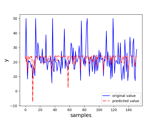
【sklearn 实现】

以 sklearn 中的波士顿房价数据集为例，选取该数据集中的 CRIM 特征作为自变量，选用普通最小二乘法实现一元线性回归

import numpy as np
import pandas as pd
import matplotlib.pyplot as plt
from sklearn.datasets import load_boston
from sklearn.model_selection import train_test_split
from sklearn.linear_model import LinearRegression
from sklearn.metrics import mean_squared_error
from sklearn.metrics import mean_squared_error
from sklearn.metrics import mean_absolute_error
from sklearn.metrics import r2_score

# 特征提取
def deal_data():
    boston = load_boston()  # sklearn的波士顿房价数据集
    df = pd.DataFrame(boston.data, columns=boston.feature_names)
    df['result'] = boston.target
    data = np.array(df)
    return data[:, 0], data[:, -1]

# 模型训练
def train_model(features, labels):
    # 由一维变为二维
    features = features.reshape(-1,1)
    labels = labels.reshape(-1,1)
    
    # 建立线性回归模型
    model = LinearRegression()
    
    # 训练
    model.fit(features, labels)
    
    return model

# 模型评估
def estimate_model(y_true, y_pred):
    MSE = mean_squared_error(y_true, y_pred)
    RMSE = np.sqrt(MSE)
    MAE = mean_absolute_error(y_true, y_pred)
    R2 = r2_score(y_true, y_pred)
    indicators = {"MSE": MSE, "RMSE":RMSE, "MAE":MAE, "R2":R2}
    return indicators

# 可视化
def visualization(y_true, y_pred, model):
    # 绘图
    plt.plot(range(y_true.shape[0]), y_true, "b-") 
    plt.plot(range(y_true.shape[0]), y_pred, "r-.")
    plt.legend(["original value", "predicted value"])
    plt.xlabel("samples", fontsize="15")
    plt.ylabel("y", fontsize="15")
    
    plt.show()

if __name__ == "__main__":
    # 特征提取
    x, y = deal_data()
    
    # 简单交叉验证
    x_train, x_test, y_train, y_test = train_test_split(x, y, test_size=0.3, random_state=0)
    
    # 模型训练
    model = train_model(x_train, y_train)
    
    # 预测结果
    x_test = x_test.reshape(-1,1) # 由一维变为二维
    y_pred = model.predict(x_test) # predict()输入输出均为二维
    y_pred = y_pred.flatten() # 由二维变为一维
    print("y test:", y_test[:10]) # 测试集y值
    print("y pred:", y_pred[:10]) # 预测y值
    
    # 模型评估
    indicators = estimate_model(y_test, y_pred)
    print("MSE:", indicators["MSE"])
    print("RMSE:", indicators["RMSE"])
    print("MAE:", indicators["MAE"])
    print("R2:", indicators["R2"])
    
    # 可视化
    visualization(y_test, y_pred, model)