References:
【GBDT 梯度提升决策树】
梯度提升决策树(Gradient Boosting Decision Tree,GBDT)是 Boosting 算法族的一种,其可认为是学习算法采用梯度提升法的提升树
- 关于梯度提升法,详见:Boosting 提升法
- 关于提升树,详见:提升树
【GBDT 回归算法】
CART 回归树
对于回归问题,设给定的容量为 $n$ 的训练集 $D=\{(\mathbf{x}_1,y_1),(\mathbf{x}_2,y_2),…,(\mathbf{x}_n,y_n)\}$,第 $i$ 组样本中的输入 $\mathbf{x}_i$ 具有 $m$ 个特征值,即:$\mathbf{x}_i=(x_i^{(1)},x_i^{(2)},…,x_i^{(m)})\in \mathbb{R}^m$,输出 $y_i\in\mathcal{Y}=\{-1,+1\}$
依照 CART 回归树,将输入空间 $\mathcal{X}$ 划分为 $K$ 个互不相交的区域 $R_1,R_2,\cdots,R_K$,并且在每个区域上确定输出的常量 $c_k$,那么决策树可表示为:
其中,$K$ 为回归树的复杂度即叶结点个数,$\{(R_1,c_1),(R_2,c_2),\cdots,(R_K,c_K)\}$ 为树的区域划分和各区域上的最优值
关于 CART 回归树,详见:决策树的 CART 生成算法
梯度提升法
对于梯度提升决策树,使用梯度提升法进行学习,即:
对于梯度提升法的第 $t$ 轮来说,给定当前模型 $G_{t-1}(\mathbf{x})$,需求解:
得到第 $t$ 棵树的参数,即第 $t$ 棵树的区域划分和各区域上的最优值
由于采用梯度提升法,因此只需要简单地拟合当前模型的负梯度 $\triangledown G_t(\mathbf{x}) = \Big[- \frac{\partial L(y,G(\mathbf{x}))}{\partial G(\mathbf{x})} \Big]_{G(\mathbf{x})=G_{t-1}(\mathbf{x})}$ 即可
算法流程
下面给出回归问题的 GBDT 算法的算法流程
输入:容量为 $n$ 的训练集 $D=\{(\mathbf{x}_1,y_1),(\mathbf{x}_2,y_2),…,(\mathbf{x}_n,y_n)\}$,第 $i$ 组样本中的输入 $\mathbf{x}_i$ 具有 $m$ 个特征值,即:$\mathbf{x}_i=(x_i^{(1)},x_i^{(2)},…,x_i^{(m)})\in \mathbb{R}^m$,输出 $y_i\in\mathcal{Y}\subset \mathbb{R}$
输出:梯度提升树 $f(\mathbf{x})$
Step1:初始化 $G_0(\mathbf{x})$
此时,$c$ 为根结点上的最优值
Step2:对 $t=1,2,\cdots,T$
1)计算负梯度
2)根据 CART 算法,对负梯度 $\triangledown G_{ti}(\mathbf{x}) $ 学习一个回归树,得到树的区域划分 $\{R_{t1},R_{t2},\cdots,R_{tK}\}$
3)根据树的区域划分 $R_{tk}$ ,计算各区域上的最优值 $\{c_{t1},c_{t2},\cdots,c_{tK}\}$
4)更新回归决策树
Step3:根据加法模型得到最终的梯度提升树
【GBDT 分类算法】
分类问题的 GBDT 算法思想上来说与回归问题 GBDT 算法没有区别,但是由于分类问题样本输出不是连续的值,而是离散的类别,这导致无法直接从输出类别去拟合类别输出的误差
为了解决这个问题,主要有两个方法:
- 使用指数损失函数:此时 GBDT 算法退化为 AdaBoost 算法
- 使用对数损失函数:用类别的预测概率值和真实概率的差来拟合损失
关于 AdaBoost 分类算法,详见:AdaBoost 算法
【GBDT 的正则化】
为防止过拟合,GBDT 与 AdaBoost 一样,需要进行正则化
GBDT 的正则化主要有三种方式:
1)对于梯度上升法的更新 $G_t(\mathbf{x}) = G_{t-1}(\mathbf{x}) + \sum\limits_{k=1}^K c_k \mathbb{I}(\mathbf{x}\in R_{tk})$,有:
其中,$\mu \in (0,1]$ 即为学习率
2)通过子采样(Subsample) 比例限制,取值 $(0,1]$
如果取值为 $1$,则说明使用全部样本,相当于没有采用子采样;如果取值小于 $1$,说明只有一部分样本会进行 GBDT 的决策树拟合
需要注意的是,这里的子采样和随机森林不一样,随机森林使用的是有放回抽样,而这里是不放回抽样
3)对弱学习器,即 CART 回归树进行正则化剪枝
【sklearn 实现】
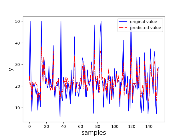
GBDT 回归算法
以 sklearn 中的波士顿房价数据集为例,选取其后两个特征来实现 GBDT 回归算法
1 | import numpy as np |
GBDT 分类算法
以 sklearn 中的鸢尾花数据集为例,选取其后两个特征来实现 AdaBoost 分类算法

1 | import pandas as pd |