Alex_McAvoy

想要成为渔夫的猎手

AdaBoost 自适应提升算法

References:

【AdaBoost 自适应提升算法】

AdaBoost 算法是自适应提升(Adaptive Boosting)算法的缩写,其是 Boosting 算法族的一种

其中,自适应(Adaptive)体现在前一个个体学习器分错的样本会得到加强,加权后的全体样本再次被用来训练下一个个体学习器,同时在每一轮中加入一个新的弱学习器,直到得到某个预定的足够小的错误率或达到预定的最大迭代次数

对于 Bootsing 提升法的加法模型:

而 AdaBoost 算法是损失函数为指数损失函数 $\exp(-yf(\mathbf{x}))$ 的 Boosting 算法

关于 Boosting 算法,详见:Boosting 提升算法

【AdaBoost 的最优化问题】

对于给定的容量为 $n$ 的训练集 $D=\{(\mathbf{x}_1,y_1),(\mathbf{x}_2,y_2),…,(\mathbf{x}_n,y_n)\}$,第 $i$ 组样本中的输入 $\mathbf{x}_i$ 具有 $m$ 个特征值,即:$\mathbf{x}_i=(x_i^{(1)},x_i^{(2)},…,x_i^{(m)})\in \mathbb{R}^m$,输出 $y_i\in\mathcal{Y}=\{+1,-1\}$,第 $t$ 轮从训练集中学习的弱学习器为 $G_t(\mathbf{x})$

假设经过 $t-1$ 轮前向分步法已经得到 $f_{t-1}(\mathbf{x})$:

在第 $t$ 轮迭代得到 $\alpha_t$ 和 $G_{t}(\mathbf{x})$,有:

那么,现在的目标是使前向分步法得到的 $\alpha_t$ 和 $G_t(\mathbf{x})$ 使 $f(\mathbf{x})$ 在训练集 $D$ 上的指数损失最小,即:

由于 $\exp[-y_if_{t-1}(\mathbf{x}_i)]$ 既不依赖于 $\alpha$,也不依赖于 $G$,因此与最小化无关,故令 $\omega_{ti}=\exp[-y_if_{t-1}(\mathbf{x}_i)]$,那么上式可表示为:

需要注意的是,$\omega_{ti}$ 依赖于 $f_{t-1}(\mathbf{x})$,其会随着每一轮的迭代而发生改变

【AdaBoost 分类算法】

参数优化

对 AdaBoost 的最优化问题:

当第 $t$ 轮从训练集中学习的弱学习器 $G_t(\mathbf{x})$ 是分类器时,考虑如何达到最小的 $\alpha_t^*$ 和 $G_t^*(\mathbf{x})$

对于 $G_t^*(\mathbf{x})$,对 $\forall \alpha>0$,使上式最小的 $G(\mathbf{x})$ 由下式可得到:

也就是说,$G_t^*(\mathbf{x})$ 是使第 $t$ 轮训练数据分类误差率最小的分类器,即为 AdaBoost 分类算法的基本分类器 $G_t(\mathbf{x})$

之后,考虑 $\alpha_t^*$,有:

将 $G_t^*(\mathbf{x})$ 带入上式,并对 $\alpha$ 求导,同时令导数为 $0$,有:

对于二分类问题来说,第 $t$ 个弱分类器 $G_t(\mathbf{x})$ 在训练集上的分类误差率为:

那么,将上式展开并化简,有:

对 $e^\alpha \text{error}_t = e^{-\alpha}(1-\text{error}_t)$ 两边同取 $\ln$,有:

可得使优化问题最小的 $\alpha$,即:

可以看出,如果分类误差率 $\text{error}_t$ 越大,那么对应的弱分类器权重系数 $\alpha_t$ 就越小,也就是说,误差率大的分类器权重系数越小

权重更新

假设第 $t$ 个弱分类器的训练集权重系数为:

那么,利用前向分步法的更新公式 $f_t(\mathbf{x})=f_{t-1}(\mathbf{x})+\alpha_t G_t(\mathbf{x})$,更新后的第 $t+1$ 个弱分类器的训练集权重系数为:

其中,$Z_t=\sum\limits_{i=1}^n \omega_{ti} \exp[-\alpha_t y_i G_t(\mathbf{x}_i)]$ 被称为规范化因子,其保证了 $D_t$ 是一个概率分布

从上式可以看出,如果第 $i$ 个样本分类错误,那么 $y_iG_t(\mathbf{x}_i)<0$,导致样本权重在第 $t+1$ 个弱分类器中增大,反之,若分类正确,那么 $y_ig_t(\mathbf{x}_i)>0$,导致样本权重在第 $t+1$ 个弱分类器中减小

分类器

最终,根据学习器的加法模型:

即可得到最终分类器:

算法流程

下面给出 AdaBoost 分类算法的算法流程

输入:对于给定的容量为 $n$ 的训练集 $D=\{(\mathbf{x}_1,y_1),(\mathbf{x}_2,y_2),…,(\mathbf{x}_n,y_n)\}$,第 $i$ 组样本中的输入 $\mathbf{x}_i$ 具有 $m$ 个特征值,即:$\mathbf{x}_i=(x_i^{(1)},x_i^{(2)},…,x_i^{(m)})\in \mathbb{R}^m$,输出 $y_i\in\mathcal{Y}=\{+1,-1\}$、弱分类算法

输出:分类学习器 $G(\mathbf{x})$

算法流程:

Step1:初始化训练集的权值分布

Step2:对 $T$ 个分类器进行迭代,即对 $t=1,2,\cdots,T$

1)使用权值分布为 $D_t$ 的训练集进行学习,得到弱分类器

2)计算第 $t$ 个弱分类器 $G_t(\mathbf{x})$ 上的分类误差率

3)计算第 $t$ 个弱分类器 $G_t(\mathbf{x})$ 的系数

4)更新第 $t+1$ 轮的训练集的权值分布

Step3:构建弱分类器的加法模型

Step4:得到最终分类器

【AdaBoost 回归算法】

AdaBoost 回归算法的推导流程与 AdaBoost 分类算法类似,这里不再给出

下面直接给出 AdaBoost 回归算法的算法流程:

输入:对于给定的容量为 $n$ 的训练集 $D=\{(\mathbf{x}_1,y_1),(\mathbf{x}_2,y_2),…,(\mathbf{x}_n,y_n)\}$,第 $i$ 组样本中的输入 $\mathbf{x}_i$ 具有 $m$ 个特征值,即:$\mathbf{x}_i=(x_i^{(1)},x_i^{(2)},…,x_i^{(m)})\in \mathbb{R}^m$,输出 $y_i\in\mathcal{Y}$、弱回归算法

输出:回归学习器 $G(\mathbf{x})$

算法流程:

Step1:初始化训练集的权值分布

Step2:对 $T$ 个分类器进行迭代,即对 $t=1,2,\cdots,T$

1)使用权值分布为 $D_t$ 的训练集进行学习,得到弱回归器

2)计算第 $t$ 个弱回归器 $G_t(\mathbf{x})$ 上的最大误差

3)根据最大误差和选用的误差计算方法,计算第 $t$ 个弱回归器 $G_t(\mathbf{x})$ 对每个样本的相对误差

  • 线性误差:$\text{error}_{ti} = \frac{|y_i-G_t(\mathbf{x}_i)|}{\text{Error}_t}$
  • 平方误差:$\text{error}_{ti} = \frac{(y_i-G_t(\mathbf{x}_i))^2}{\text{Error}_t^2}$
  • 指数误差:$\text{error}_{ti} = 1-\exp[\frac{-y_i+G_t(\mathbf{x}_i)}{\text{Error}_t}]$

4)计算第 $t$ 个弱回归器 $G_t(\mathbf{x})$ 的回归误差率

5)计算第 $t$ 个弱回归器 $G_t(\mathbf{x})$ 的系数

6)更新第 $t+1$ 轮的训练集的权值分布

Step3:得到最终回归器

其中,$g(\mathbf{x})$ 为所有 $\alpha_tG_t(\mathbf{x})$ 的中位数

【AdaBoost 的正则化】

通常来说,为防止 AdaBoost 出现过拟合,会加入正则化项,这个正则化项即学习率(Learning Rate)

对于前向分步法的更新公式的 $f_t(\mathbf{x})=f_{t-1}(\mathbf{x})+\alpha_t G_t(\mathbf{x})$,有:

其中,$\mu\in(0,1]$ 即为学习率

对于同样的训练集来说,较小的 $\mu$ 意味着需要更多的弱学习器的迭代次数,通常用学习率和迭代最大次数来一起决定算法的拟合效果
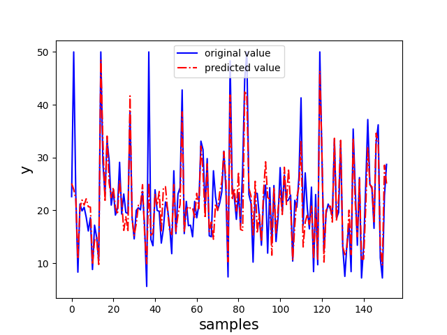
【sklearn 实现】

GBDT 回归算法

sklearn 中的波士顿房价数据集为例,选取其后两个特征来实现 AdaBoost 回归算法

1
2
3
4
5
6
7
8
9
10
11
12
13
14
15
16
17
18
19
20
21
22
23
24
25
26
27
28
29
30
31
32
33
34
35
36
37
38
39
40
41
42
43
44
45
46
47
48
49
50
51
52
53
54
55
56
57
58
59
60
61
62
63
64
65
66
67
68
69
70
71
72
73
import numpy as np
import pandas as pd
import matplotlib.pyplot as plt
from sklearn.datasets import load_boston
from sklearn.model_selection import train_test_split
from sklearn.ensemble import AdaBoostRegressor
from sklearn.tree import DecisionTreeRegressor
from sklearn.metrics import mean_squared_error
from sklearn.metrics import mean_absolute_error
from sklearn.metrics import r2_score

# 特征提取
def deal_data():
boston = load_boston() # sklearn的波士顿房价数据集
df = pd.DataFrame(boston.data, columns=boston.feature_names)
df['result'] = boston.target
data = np.array(df)
return data[:, :-1], data[:, -1]

# 模型训练
def train_model(features, labels):
# 建立AdaBoost回归模型
model = AdaBoostRegressor(base_estimator=DecisionTreeRegressor(max_depth=4),
n_estimators=300)

# 训练
model.fit(features, labels)
return model

# 模型评估
def estimate_model(y_true, y_pred):
MSE = mean_squared_error(y_true, y_pred)
RMSE = np.sqrt(MSE)
MAE = mean_absolute_error(y_true, y_pred)
R2 = r2_score(y_true, y_pred)
indicators = {"MSE": MSE, "RMSE":RMSE, "MAE":MAE, "R2":R2}
return indicators

# 可视化
def visualization(y_true, y_pred, model):
# 绘图
plt.plot(range(y_true.shape[0]), y_true, "b-")
plt.plot(range(y_true.shape[0]), y_pred, "r-.")
plt.legend(["original value", "predicted value"])
plt.xlabel("samples", fontsize="15")
plt.ylabel("y", fontsize="15")

plt.show()

if __name__ == "__main__":
# 特征提取
x, y = deal_data()

# 简单交叉验证
x_train, x_test, y_train, y_test = train_test_split(x, y, test_size=0.3, random_state=0)

# 模型训练
model = train_model(x_train, y_train)

# 预测结果
y_pred = model.predict(x_test) # predict()输入输出均为二维
print("y test:", y_test[:10]) # 测试集y值
print("y pred:", y_pred[:10]) # 预测y值

# 模型评估
indicators = estimate_model(y_test, y_pred)
print("MSE:", indicators["MSE"])
print("RMSE:", indicators["RMSE"])
print("MAE:", indicators["MAE"])
print("R2:", indicators["R2"])

# 可视化
visualization(y_test, y_pred, model)

GBDT 分类算法

sklearn 中的鸢尾花数据集为例,选取其后两个特征来实现 AdaBoost 分类算法

1
2
3
4
5
6
7
8
9
10
11
12
13
14
15
16
17
18
19
20
21
22
23
24
25
26
27
28
29
30
31
32
33
34
35
36
37
38
39
40
41
42
43
44
45
46
47
48
49
50
51
52
53
54
55
56
57
58
59
60
61
62
63
64
65
66
67
68
69
70
71
72
73
74
75
76
77
78
79
80
81
82
83
84
85
86
87
88
89
90
91
92
93
94
95
96
97
98
99
100
101
102
103
104
105
106
107
108
109
110
111
112
113
114
115
116
117
118
119
120
121
122
123
124
125
126
127
128
129
130
131
import pandas as pd
import numpy as np
import matplotlib.pyplot as plt
from sklearn.datasets import load_iris
from sklearn.model_selection import train_test_split
from sklearn.preprocessing import StandardScaler
from sklearn.tree import DecisionTreeClassifier
from sklearn.ensemble import AdaBoostClassifier
from sklearn.metrics import confusion_matrix,accuracy_score,classification_report,precision_score,recall_score,f1_score
from matplotlib.colors import ListedColormap

# 特征提取
def deal_data():
iris = load_iris() # sklearn的鸢尾花数据集
# iris分为三类,前50行一类,51-100行一类,101-150行一类
X = iris.data[:, [2, 3]] # 选用后两个特征作为样本特征
y = iris.target #取species列,类别
return X,y

# 数据归一化
def standard_scaler(X_train,X_test):
sc = StandardScaler() # 初始化一个sc对象去对数据集作变换
scaler = sc.fit(X_train) # 归一化,存有计算出的均值和方差
X_train_std = scaler.transform(X_train) # 利用 scaler 进行标准化
X_test_std = scaler.transform(X_test) # 利用 scaler 进行标准化
return X_train_std, X_test_std

# 模型训练
def train_model(X_train_std, y_train):
# 建立AdaBoost分类模型
# - algorithm:samme输出分类的标签,samme.R输出分类的概率
# - n_estimators:基学习器数量
# - learning_rate:学习率
model = AdaBoostClassifier(base_estimator=DecisionTreeClassifier(), algorithm="SAMME", n_estimators=200, learning_rate=0.8)
# 训练
model.fit(X_train_std, y_train)
return model

# 模型评估
def estimate_model(y_pred, y_test, model):
# 混淆矩阵,三分类情况下,大小为 3*3
cm2 = confusion_matrix(y_test,y_pred)
# 准确率
acc = accuracy_score(y_test,y_pred)
# 正确分类的样本数
acc_num = accuracy_score(y_test,y_pred,normalize=False)
# macro 分类报告
macro_class_report = classification_report(y_test, y_pred,target_names=["类0","类1","类2"])
# 微精确率
micro_p = precision_score(y_test,y_pred,average='micro')
# 微召回率
micro_r = recall_score(y_test,y_pred,average='micro')
# 微F1得分
micro_f1 = f1_score(y_test,y_pred,average='micro')

indicators = {"cm2":cm2,"acc":acc,"acc_num":acc_num,"macro_class_report":macro_class_report,"micro_p":micro_p,"micro_r":micro_r,"micro_f1":micro_f1}
return indicators

# 可视化
def visualization(X, y, classifier, test_id=None, resolution=0.02):
# 创建 color map
markers = ('s', 'x', 'o', '^', 'v')
colors = ('red', 'blue', 'lightgreen', 'gray', 'cyan')
cmap = ListedColormap(colors[:len(np.unique(y))])

# 绘制决策边界
x1_min, x1_max = X[:, 0].min() - 1, X[:, 0].max() + 1 #第一个特征取值范围作为横轴
x2_min, x2_max = X[:, 1].min() - 1, X[:, 1].max() + 1 #第二个特征取值范围作为纵轴
xx1, xx2 = np.meshgrid(np.arange(x1_min, x1_max, resolution), np.arange(x2_min, x2_max, resolution)) # reolution为网格剖分粒度
Z = classifier.predict(np.array([xx1.ravel(), xx2.ravel()]).T) # 对组合的特征进行预测,ravel为数组展平
Z = Z.reshape(xx1.shape) # Z是列向量
plt.contourf(xx1, xx2, Z, alpha=0.4, cmap=cmap) # x和y为两个等长一维数组,z为二维数组,指定每一对xy所对应的z值
plt.xlim(xx1.min(), xx1.max()) #对等高线间的区域进行填充
plt.ylim(xx2.min(), xx2.max()) #对等高线间的区域进行填充

# 全数据集,不同类别样本点的特征作为坐标(x,y),用不同颜色画散点图
for idx, cl in enumerate(np.unique(y)):
plt.scatter(x=X[y == cl, 0], y=X[y == cl, 1], alpha=0.8, c=cmap(idx), marker=markers[idx], label=cl)

# 高亮测试集
if test_id:
X_test, y_test = X[test_id, :], y[test_id]
# c设置颜色,测试集不同类别的实例点画图不区别颜色
plt.scatter(x=X_test[:, 0], y=X_test[:, 1], alpha=1.0, c='gray', marker='^', linewidths=1, s=55, label='test set')

plt.xlabel('petal length [standardized]')
plt.ylabel('petal width [standardized]')
plt.legend(loc='upper left')
plt.tight_layout()
plt.show()

if __name__ == "__main__":
# 特征提取
X, y = deal_data()

# 简单交叉验证
X_train, X_test, y_train, y_test = train_test_split(X, y, test_size=0.3, random_state=0)

# 数据标准化
X_train_std, X_test_std = standard_scaler(X_train, X_test)

# 模型训练
model = train_model(X_train_std, y_train)

# 预测结果
y_pred = model.predict(X_test_std)
print("y test:", y_test) # 测试集y值
print("y pred:", y_pred) # 预测y值

# 模型评估
indicators = estimate_model(y_pred, y_test, model)
cm2 = indicators["cm2"]
print("混淆矩阵:\n", cm2)
acc = indicators["acc"]
print("准确率:", acc)
acc_num = indicators["acc_num"]
print("正确分类的样本数:", acc_num)
macro_class_report = indicators["macro_class_report"]
print("macro 分类报告:\n", macro_class_report)
micro_p = indicators["micro_p"]
print("微精确率:", micro_p)
micro_r = indicators["micro_r"]
print("微召回率:", micro_r)
micro_f1 = indicators["micro_f1"]
print("微F1得分:", micro_f1)

# 可视化
X_combined_std = np.vstack((X_train_std, X_test_std))
y_combined = np.hstack((y_train, y_test))
# classifier为分类器,test_id为测试集序号
visualization(X_combined_std, y_combined, classifier=model, test_id=range(105, 150))
感谢您对我的支持,让我继续努力分享有用的技术与知识点!