【决策树】

决策树（Decision Tree）是一种用于分类或回归的机器学习方法，对于复杂的预测问题，通过建立树模型产生分支结点，依照规则递归地分割数据集，使得问题从结构上划分为不同的子问题

决策树本质是从训练集中归纳出一组规则，在给出一个新的输入后，根据规则给出相应的输出，由于与训练集不矛盾的决策树可能有多个，需要选择一个与训练数据矛盾较小的决策树，同时具有较好的泛化能力

从另一个角度来看，决策树是由训练集估计的条件概率模型，而基于特征空间划分的条件概率模型有无穷多个，选择的条件概率模型不仅要对训练数据有很好的拟合，而且对未知数据有很好的预测

根据所处理数据的类型，决策树可以分为以下两种：

• 分类决策树：处理的数据是离散值，用来解决分类问题
• 回归决策树：处理的数据是连续值，用来解决回归问题

此外，还有一种由 CART 决策树生成算法构建的分类与回归树（Classification and Regression Trees），其既可以处理分类问题，也可以处理回归问题

【结构】

一般地，一棵决策树包含一个根结点、若干分支结点、若干叶结点

其中，根结点包含样本全集，叶结点对应决策结果，分支结点对应于一个属性测试

从根结点到每个叶结点的路径对应了一个判定测试序列（if-then 规则），路径上的分支结点的特征对应着规则的条件，叶结点对应着规则的结论

随着树深度不断地增加，分支结点的子集会越来越小，问题也逐渐简化，当分支结点的深度或问题的规模满足一定的停止条件时，分支结点会停止分裂

举例来说，为了预测明天是否适合出去打羽毛球，采集了过去 14 天的数据，数据特征包括天气、温度、湿度、风力，如下表所示：

下图是可能的决策树分裂方案之一：

其中，根结点是天气，分支结点是湿度、风力，叶结点是适合、不适合

【sklearn 实现】

sklearn.tree

在 sklearn.tree 中，存在两个关于决策树的方法，这两种方法所采用的算法都是 CART 算法，一个用来处理回归问题，另一个用来处理分类问题：

• DecisionTreeRegressor()：处理回归问题
• DecisionTreeClassifier()：处理分类问题

两个方法的参数一致，使用方法相似，二者唯一的区别是用于处理分类问题的 DecisionTreeClassifier() 相较于 DecisionTreeRegressor() 多了一个 class_weight 参数

决策树结构可视化

sklearn 中没有提供决策树的可视化，其仅能让训练的模型保存到 dot 文件中

from sklearn.tree import export_graphviz
with open("out.dot", "w") as f:
    f = export_graphviz(model, out_file = f, 
                        feature_names = ['a', 'b', 'c', 'd'])

之后，一般使用 graphviz 来进行可视化，其部署主要包括 graphviz 的安装和 Python 的 graphviz 插件的安装

1. 安装 graphviz：点击这里
2. 设置环境变量：将 安装目录/Graphviz/bin 加入 PATH 中
3. 安装 graphviz 插件：pip install graphviz
4. 安装 pydotplus 插件： pip install pydotplus

此时，环境配置完成，若仍然找不到 graphviz，加入以下代码即可：

import os
os.environ["PATH"] += os.pathsep + "安装目录/Graphviz/bin/"

有两种方法生成决策树的可视化

方案一：生成 pdf

import pydotplus 
from sklearn.tree import export_graphviz
dot_data = export_graphviz(model, out_file=None) 
graph = pydotplus.graph_from_dot_data(dot_data) 
graph.write_pdf("out.pdf")

方案二：直接在 Jupyter 中显示

from IPython.display import Image  
from sklearn.tree import export_graphviz
import pydotplus 
import os

os.environ["PATH"] += os.pathsep + "安装目录/Graphviz/bin/"
dot_data = export_graphviz(model, out_file=None, 
                         feature_names=['a', 'b', 'c', 'd'],  
                         class_names=['calss1','calss2','calss3'],  
                         filled=True, rounded=True,  
                         special_characters=True)  

graph = pydotplus.graph_from_dot_data(dot_data)  
Image(graph.create_png())

实现

以 sklearn 中的鸢尾花数据集为例，选取其后两个特征来实现决策树

import pandas as pd
import numpy as np
import matplotlib.pyplot as plt
from sklearn.datasets import load_iris
from sklearn.model_selection import train_test_split
from sklearn.preprocessing import StandardScaler
from sklearn.tree import DecisionTreeClassifier
from sklearn.metrics import confusion_matrix,accuracy_score,classification_report,precision_score,recall_score,f1_score
from matplotlib.colors import ListedColormap

# 特征提取
def deal_data():
    iris = load_iris()  # sklearn的鸢尾花数据集
    # iris分为三类，前50行一类，51-100行一类，101-150行一类
    X = iris.data[:, [2, 3]] # 选用后两个特征作为样本特征
    y = iris.target  #取species列，类别
    return X,y

# 数据归一化
def standard_scaler(X_train,X_test):
    sc = StandardScaler() # 初始化一个sc对象去对数据集作变换
    scaler = sc.fit(X_train) # 归一化，存有计算出的均值和方差
    X_train_std = scaler.transform(X_train) # 利用 scaler 进行标准化
    X_test_std = scaler.transform(X_test) # 利用 scaler 进行标准化
    return X_train_std, X_test_std

# 模型训练
def train_model(X_train_std, y_train):
    # 建立决策树模型
    model = DecisionTreeClassifier(criterion='entropy', max_depth=4)
    # 训练
    model.fit(X_train_std, y_train)
    return model

# 模型评估
def estimate_model(y_pred, y_test, model):
    # 混淆矩阵，三分类情况下，大小为 3*3
    cm2 = confusion_matrix(y_test,y_pred) 
    # 准确率
    acc = accuracy_score(y_test,y_pred)
    # 正确分类的样本数
    acc_num = accuracy_score(y_test,y_pred,normalize=False)
    # macro 分类报告
    macro_class_report = classification_report(y_test, y_pred,target_names=["类0","类1","类2"])
    # 微精确率
    micro_p = precision_score(y_test,y_pred,average='micro') 
    # 微召回率
    micro_r = recall_score(y_test,y_pred,average='micro')
    # 微F1得分
    micro_f1 = f1_score(y_test,y_pred,average='micro') 
    
    indicators = {"cm2":cm2,"acc":acc,"acc_num":acc_num,"macro_class_report":macro_class_report,"micro_p":micro_p,"micro_r":micro_r,"micro_f1":micro_f1}
    return indicators
    
# 可视化
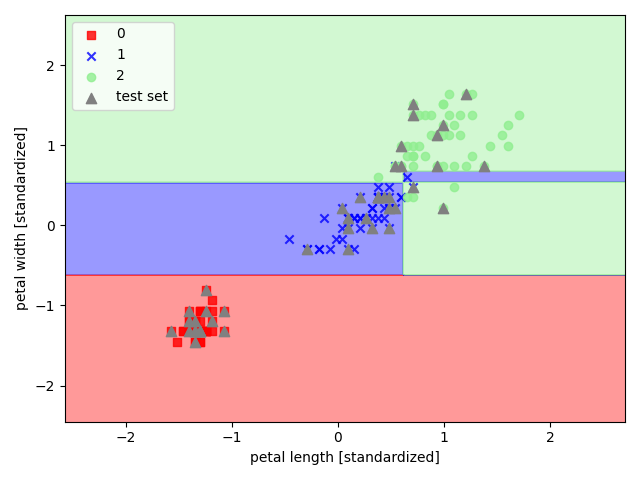
def visualization(X, y, classifier, test_id=None, resolution=0.02):
    # 创建 color map
    markers = ('s', 'x', 'o', '^', 'v')
    colors = ('red', 'blue', 'lightgreen', 'gray', 'cyan')
    cmap = ListedColormap(colors[:len(np.unique(y))])
    
    # 绘制决策边界
    x1_min, x1_max = X[:, 0].min() - 1, X[:, 0].max() + 1 #第一个特征取值范围作为横轴
    x2_min, x2_max = X[:, 1].min() - 1, X[:, 1].max() + 1 #第二个特征取值范围作为纵轴
    xx1, xx2 = np.meshgrid(np.arange(x1_min, x1_max, resolution), np.arange(x2_min, x2_max, resolution)) # reolution为网格剖分粒度
    Z = classifier.predict(np.array([xx1.ravel(), xx2.ravel()]).T) # 对组合的特征进行预测，ravel为数组展平
    Z = Z.reshape(xx1.shape) # Z是列向量
    plt.contourf(xx1, xx2, Z, alpha=0.4, cmap=cmap) # x和y为两个等长一维数组，z为二维数组，指定每一对xy所对应的z值
    plt.xlim(xx1.min(), xx1.max()) #对等高线间的区域进行填充
    plt.ylim(xx2.min(), xx2.max()) #对等高线间的区域进行填充
    
    # 全数据集，不同类别样本点的特征作为坐标(x,y)，用不同颜色画散点图
    for idx, cl in enumerate(np.unique(y)):
        plt.scatter(x=X[y == cl, 0], y=X[y == cl, 1], alpha=0.8, c=cmap(idx), marker=markers[idx], label=cl) 
        
    # 高亮测试集
    if test_id:
        X_test, y_test = X[test_id, :], y[test_id]
        # c设置颜色，测试集不同类别的实例点画图不区别颜色
        plt.scatter(x=X_test[:, 0], y=X_test[:, 1], alpha=1.0, c='gray', marker='^', linewidths=1, s=55, label='test set')

    plt.xlabel('petal length [standardized]')
    plt.ylabel('petal width [standardized]')
    plt.legend(loc='upper left')
    plt.tight_layout()
    plt.show()

# 可视化决策树结构
def visualization_tree(way = "pdf"):
    from sklearn.tree import export_graphviz
    import pydotplus

    # 生成pdf文件
    if way == "pdf":
        # 将模型保存为dot文件
        with open("out.dot", "w") as f:
            f = export_graphviz(model, out_file = f, 
                                feature_names = ["petal length", "petal width"])
        # 将dot文件进行可视化，存为pdf
        dot_data = export_graphviz(model, out_file=None) 
        graph = pydotplus.graph_from_dot_data(dot_data) 
        graph.write_pdf("out.pdf") 
    
    # 在jupyter中可视化
    if way == "jupyter":
        from IPython.display import Image  
        import os
        
        os.environ["PATH"] += os.pathsep + "I:/Graphviz/bin/"
        dot_data = export_graphviz(model, out_file=None, 
                                 feature_names=["petal length", "petal width"],  
                                 filled=True, rounded=True,  
                                 special_characters=True)  

        graph = pydotplus.graph_from_dot_data(dot_data)  
        return Image(graph.create_png())

if __name__ == "__main__":
    # 特征提取
    X, y = deal_data()
    
    # 简单交叉验证
    X_train, X_test, y_train, y_test = train_test_split(X, y, test_size=0.3, random_state=0)
    
    # 数据标准化
    X_train_std, X_test_std = standard_scaler(X_train, X_test)
    
    # 模型训练
    model = train_model(X_train_std, y_train)
    
    # 预测结果
    y_pred = model.predict(X_test_std)
    print("y test:", y_test) # 测试集y值
    print("y pred:", y_pred) # 预测y值
    
    # 模型评估
    indicators = estimate_model(y_pred, y_test, model)
    cm2 = indicators["cm2"] 
    print("混淆矩阵：\n", cm2) 
    acc =  indicators["acc"]
    print("准确率：", acc)
    acc_num =  indicators["acc_num"]
    print("正确分类的样本数：", acc_num)
    macro_class_report = indicators["macro_class_report"]
    print("macro 分类报告：\n", macro_class_report)
    micro_p = indicators["micro_p"]
    print("微精确率：", micro_p)
    micro_r = indicators["micro_r"]
    print("微召回率：", micro_r)
    micro_f1 = indicators["micro_f1"]
    print("微F1得分：", micro_f1)
    
    # 可视化
    X_combined_std = np.vstack((X_train_std, X_test_std))
    y_combined = np.hstack((y_train, y_test))
    # classifier为分类器，test_id为测试集序号
    visualization(X_combined_std, y_combined, classifier=model, test_id=range(105, 150))
    
    # 可视化决策树结构
    visualization_tree("pdf")