1
2
3
4
5
6
7
8
9
10
11
12
13
14
15
16
17
18
19
20
21
22
23
24
25
26
27
28
29
30
31
32
33
34
35
36
37
38
39
40
41
42
43
44
45
46
47
48
49
50
51
52
53
54
55
56
57
58
59
60
61
62
63
64
65
66
67
68
69
70
71
72
73
74
75
76
77
78
79
80
81
82
83
84
85
86
87
88
89
90
91
92
93
94
95
96
97
98
99
100
101
102
103
104
105
106
107
108
109
110
111
112
113
114
115
116
117
118
119
120
121
122
123
124
125
126
127
128
129
130
131
132
133
134
135
136
137
138
139
140
141
142
143
144
145
146
147
148
149
150
151
152
153
154
155
156
157
158
159
160
161
162
163
164
165
166
167
168
169
170
171
172
173
174
175
176
177
178
179
180
181
182
183
184
185
186
187
188
189
190
191
192
193
194
195
196
197
198
199
200
201
202
203
204
205
206
207
208
209
210
211
212
213
214
215
216
217
218
219
220
221
222
223
224
225
226
227
228
229
230
231
232
233
234
235
236
237
238
239
240
241
| import numpy as np
import pandas as pd
import matplotlib.pyplot as plt
from collections import defaultdict
import math
from sklearn.datasets import load_iris
from sklearn.model_selection import train_test_split
from sklearn.preprocessing import StandardScaler
from sklearn.metrics import confusion_matrix,accuracy_score,classification_report,precision_score,recall_score,f1_score
from matplotlib.colors import ListedColormap
def deal_data():
iris = load_iris()
X = iris.data[:, [2, 3]]
y = iris.target
return X,y
def standard_scaler(X_train,X_test):
sc = StandardScaler()
scaler = sc.fit(X_train)
X_train_std = scaler.transform(X_train)
X_test_std = scaler.transform(X_test)
return X_train_std, X_test_std
def features_rebuild(old_features):
'''
最大熵模型f(x,y)中的x是一个单独的特征,不是n维特征向量
为此,要对每个维度加一个区分特征
具体来说,将原来feature的(a0,a1,a2,...)变成(0_a0,1_a1,2_a2,...)的形式
'''
new_features = []
for feature in old_features:
new_feature = []
for i, f in enumerate(feature):
new_feature.append(str(i) + '_' + str(f))
new_features.append(new_feature)
return new_features
class MaxEnt(object):
def init_params(self, X, Y):
self.X_ = X
self.Y_ = set()
self.cal_Vxy(X, Y)
self.N = len(X)
self.n = len(self.Vxy)
self.M = 10000.0
self.build_dict()
self.cal_pxy()
def build_dict(self):
self.id2xy = {}
self.xy2id = {}
for i, (x, y) in enumerate(self.Vxy):
self.id2xy[i] = (x, y)
self.xy2id[(x, y)] = i
def cal_Vxy(self, X, Y):
self.Vxy = defaultdict(int)
for i in range(len(X)):
x_, y = X[i], Y[i]
self.Y_.add(y)
for x in x_:
self.Vxy[(x, y)] += 1
def cal_pxy(self):
self.pxy = defaultdict(float)
for id in range(self.n):
(x, y) = self.id2xy[id]
self.pxy[id] = float(self.Vxy[(x, y)]) / float(self.N)
def cal_Zx(self, X, y):
result = 0.0
for x in X:
if (x,y) in self.xy2id:
id = self.xy2id[(x, y)]
result += self.w[id]
return (math.exp(result), y)
def cal_pyx(self, X):
pyxs = [(self.cal_Zx(X, y)) for y in self.Y_]
Zwx = sum([prob for prob, y in pyxs])
return [(prob / Zwx, y) for prob, y in pyxs]
def cal_Epfi(self):
self.Epfi = [0.0 for i in range(self.n)]
for i, X in enumerate(self.X_):
pyxs = self.cal_pyx(X)
for x in X:
for pyx, y in pyxs:
if (x,y) in self.xy2id:
id = self.xy2id[(x, y)]
self.Epfi[id] += pyx * (1.0 / self.N)
def fit(self, X, Y):
self.init_params(X, Y)
max_iteration = 500
self.w = [0.0 for i in range(self.n)]
for times in range(max_iteration):
detas = []
self.cal_Epfi()
for i in range(self.n):
deta = 1 / self.M * math.log(self.pxy[i] / self.Epfi[i])
detas.append(deta)
self.w = [self.w[i] + detas[i] for i in range(self.n)]
def predict(self, testset):
results = []
for test in testset:
result = self.cal_pyx(test)
results.append(max(result, key=lambda x: x[0])[1])
return results
def train_model(X_train_std, y_train):
model = MaxEnt()
model.fit(X_train_std, y_train)
return model
def estimate_model(y_pred, y_test, model):
cm2 = confusion_matrix(y_test,y_pred)
acc = accuracy_score(y_test,y_pred)
acc_num = accuracy_score(y_test,y_pred,normalize=False)
macro_class_report = classification_report(y_test, y_pred,target_names=["类0","类1","类2"])
micro_p = precision_score(y_test,y_pred,average='micro')
micro_r = recall_score(y_test,y_pred,average='micro')
micro_f1 = f1_score(y_test,y_pred,average='micro')
indicators = {"cm2":cm2,"acc":acc,"acc_num":acc_num,"macro_class_report":macro_class_report,"micro_p":micro_p,"micro_r":micro_r,"micro_f1":micro_f1}
return indicators
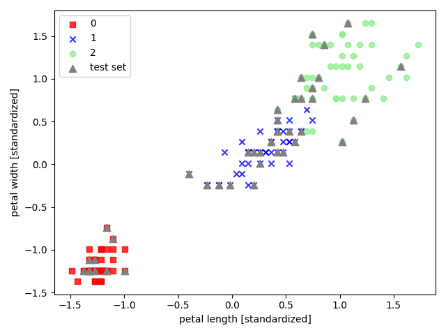
def visualization(X, y, classifier, test_id=None, resolution=0.02):
for i in range(0,150):
X[i][0] = X[i][0].replace("0_","")
X[i][1] = X[i][1].replace("1_","")
X = X.astype(float)
markers = ('s', 'x', 'o', '^', 'v')
colors = ('red', 'blue', 'lightgreen', 'gray', 'cyan')
cmap = ListedColormap(colors[:len(np.unique(y))])
for idx, cl in enumerate(np.unique(y)):
plt.scatter(x=X[y == cl, 0], y=X[y == cl, 1], alpha=0.8, c=cmap(idx), marker=markers[idx], label=cl)
if test_id:
X_test, y_test = X[test_id, :], y[test_id]
plt.scatter(x=X_test[:, 0], y=X_test[:, 1], alpha=1.0, c='gray', marker='^', linewidths=1, s=55, label='test set')
plt.xlabel('petal length [standardized]')
plt.ylabel('petal width [standardized]')
plt.legend(loc='upper left')
plt.tight_layout()
plt.show()
if __name__ == '__main__':
X, y = deal_data()
X_train, X_test, y_train, y_test = train_test_split(X, y, test_size=0.3)
X_train_std, X_test_std = standard_scaler(X_train, X_test)
X_train_std = features_rebuild(X_train_std)
X_test_std = features_rebuild(X_test_std)
model = train_model(X_train_std, y_train)
y_pred = model.predict(X_test_std)
print("y test:", y_test)
print("y pred:", y_pred)
indicators = estimate_model(y_pred, y_test, model)
cm2 = indicators["cm2"]
print("混淆矩阵:\n", cm2)
acc = indicators["acc"]
print("准确率:", acc)
acc_num = indicators["acc_num"]
print("正确分类的样本数:", acc_num)
macro_class_report = indicators["macro_class_report"]
print("macro 分类报告:\n", macro_class_report)
micro_p = indicators["micro_p"]
print("微精确率:", micro_p)
micro_r = indicators["micro_r"]
print("微召回率:", micro_r)
micro_f1 = indicators["micro_f1"]
print("微F1得分:", micro_f1)
X_combined_std = np.vstack((X_train_std, X_test_std))
y_combined = np.hstack((y_train, y_test))
visualization(X_combined_std, y_combined, classifier=model, test_id=range(105, 150))
|