Alex_McAvoy

想要成为渔夫的猎手

单层感知机

【概述】

感知机(Perceptron)是神经网络和支持向量机的起源算法,从结构上来讲,其分为单层感知机(Single Layer Perceptron)多层感知机(Multi-Layer Perceptron)

单层感知机就是 MP 神经元,其一般用于处理线性可分问题,多层感知机是多个 MP 神经元的累叠,通过增加层数来处理线性不可分问题

单层感知机与 MP 神经元最主要的区别,在于感知机引入了损失函数与参数学习的过程,这是为什么将感知机称为最初的神经网络模型的原因

本文仅介绍单层感知机,为便于表述,以下内容所提到的感知机,均为单层感知机

【单层感知机模型】

假设形式

单层感知机是一种二分类的线性分类模型,其本质上是寻找特征空间 $\mathbb{R}^{n}$ 中的一个超平面 $S:\boldsymbol{\omega}\cdot \mathbf{x}+\theta=0$,将特征空间划分为两个部分,使得位于两部分的点被分为正负两类

设输入空间 $\mathcal{X}\in \mathbb{R}^{n}$,输出空间 $\mathcal{Y}=\{-1,+1\}$,输入 $\mathbf{x}=(x^{(1)},x^{(2)},…,x^{(n)})\in\mathcal{X}$ 为实例的特征向量,对应于输入空间的点,输出 $y\in\mathcal{Y}$ 为实例的类别

在感知机中,激活函数一般使用 $\text{sign}(\cdot)$ 函数:

其中,$\boldsymbol{\omega}\in \mathbb{R}^{n}$ 为权值(Weight),$\theta\in \mathbb{R}$ 为阈值(Threshold),$\boldsymbol{\omega}\cdot \mathbf{x}$ 表示 $\boldsymbol{\omega}$ 与 $\mathbf{x}$ 的内积

可以发现,感知机与 MP 神经元本质上是一致的,只是为了便于表达,将阈值 $\theta$ 取负,从而使得 $\boldsymbol{\omega}\cdot\mathbf{x}-\theta$ 的减法变为 $\boldsymbol{\omega}\cdot\mathbf{x}+\theta$ 的加法

损失函数

假设训练集是线性可分的,单层感知机学习的目标是求得一个能够将训练集正样本和负样本完全正确分开的分离超平面,为找出这样的分离超平面,即求得感知机的模型参数 $\boldsymbol{\omega}$ 和阈值 $\theta$,为此,需要定义经验损失函数并将该损失函数极小化

在感知机模型中,最直观的损失函数是误分类样本点的个数,但这样的损失函数不是 $\boldsymbol{\omega}$ 与 $\theta$ 的连续可导函数,不易优化,因此,在感知机中一般选用误分类样本点到超平面 $S$ 的总几何间隔作为损失函数

线性可分与几何间隔 中,介绍了对于分离超平面 $S:\boldsymbol{\omega}\cdot \mathbf{x}+\theta=0$ 几何间隔:

对于样本集 $D$ 中的误分类的样本 $(\mathbf{x}_j,y_j)$ 来说,有:

  • 当 $\boldsymbol{\omega}\cdot\mathbf{x}_j+\theta>0$ 时,$y_j=-1$
  • 当 $\boldsymbol{\omega}\cdot\mathbf{x}_j+\theta<0$ 时,$y_j=+1$

即:

由此,误分类样本 $(\mathbf{x}_j,y_j)$ 到超平面 $S$ 的几何间隔为:

那么,假设超平面 $S$ 的误分类点的集合为 $E$,则所有误分类点到超平面 $S$ 的总几何间隔为:

于是,对于给定训练集 $D=\{(\mathbf{x}_1,y_1),(\mathbf{x}_2,y_2),…,(\mathbf{x}_N,y_N)\}$,第 $i$ 组样本中的输入 $\mathbf{x}_i$ 具有 $n$ 个特征值,即:$\mathbf{x}_i=(x_i^{(1)},x_i^{(2)},…,x_i^{(n)})\in \mathbb{R}^n$,输出 $y_i\in\mathcal{Y}=\{+1,-1\}$

对于误分类点集 $E=\{(\mathbf{x}_1,y_1),(\mathbf{x}_2,y_2),…,(\mathbf{x}_M,y_M)\},M\leq N$,第 $j$ 组样本中的输入 $\mathbf{x}_j$ 具有 $n$ 个特征值,即:$\mathbf{x}_j=(x_i^{(1)},x_i^{(2)},…,x_i^{(n)})\in \mathbb{R}^n$,输出 $y_j\in\mathcal{Y}=\{+1,-1\}$

不考虑 $\frac{1}{||\boldsymbol{\omega}||_2} $,感知机 $f(\mathbf{x})=\text{sign}(\boldsymbol{\omega}\cdot \mathbf{x}+\theta)$ 的损失函数为:

显然,$L(\boldsymbol{\omega},\theta)$ 是非负的,若没有误分类点,则 $L(\boldsymbol{\omega},\theta)=0$,同时,误分类点越少,误分类点就距离超平面越近,损失函数值也就越小
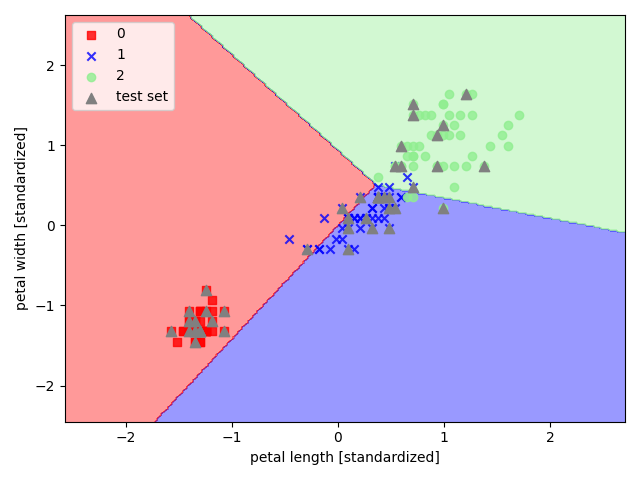
【sklearn 实现】

以 sklearn 中的鸢尾花数据集为例,选取其后两个特征来实现感知机

1
2
3
4
5
6
7
8
9
10
11
12
13
14
15
16
17
18
19
20
21
22
23
24
25
26
27
28
29
30
31
32
33
34
35
36
37
38
39
40
41
42
43
44
45
46
47
48
49
50
51
52
53
54
55
56
57
58
59
60
61
62
63
64
65
66
67
68
69
70
71
72
73
74
75
76
77
78
79
80
81
82
83
84
85
86
87
88
89
90
91
92
93
94
95
96
97
98
99
100
101
102
103
104
105
106
107
108
109
110
111
112
113
114
115
116
117
118
119
120
121
122
123
124
125
126
127
128
import pandas as pd
import numpy as np
import matplotlib.pyplot as plt
from sklearn.datasets import load_iris
from sklearn.model_selection import train_test_split
from sklearn.preprocessing import StandardScaler
from sklearn.linear_model import Perceptron
from sklearn.metrics import confusion_matrix,accuracy_score,classification_report,precision_score,recall_score,f1_score
from matplotlib.colors import ListedColormap

# 特征提取
def deal_data():
iris = load_iris() # sklearn的鸢尾花数据集
# iris分为三类,前50行一类,51-100行一类,101-150行一类
X = iris.data[:, [2, 3]] # 选用后两个特征作为样本特征
y = iris.target #取species列,类别
return X,y

# 数据归一化
def standard_scaler(X_train,X_test):
sc = StandardScaler() # 初始化一个sc对象去对数据集作变换
scaler = sc.fit(X_train) # 归一化,存有计算出的均值和方差
X_train_std = scaler.transform(X_train) # 利用 scaler 进行标准化
X_test_std = scaler.transform(X_test) # 利用 scaler 进行标准化
return X_train_std, X_test_std

# 模型训练
def train_model(X_train_std, y_train):
# 建立感知机模型
# tol参数设置一个特定值,当本次迭代损失与上次迭代损失的差小于一个特定值时,停止迭代;若设置为None,将会一直迭代,直至差为0
model = Perceptron(tol=None)
# 训练
model.fit(X_train_std, y_train)
return model

# 模型评估
def estimate_model(y_pred, y_test, model):
# 混淆矩阵,三分类情况下,大小为 3*3
cm2 = confusion_matrix(y_test,y_pred)
# 准确率
acc = accuracy_score(y_test,y_pred)
# 正确分类的样本数
acc_num = accuracy_score(y_test,y_pred,normalize=False)
# macro 分类报告
macro_class_report = classification_report(y_test, y_pred,target_names=["类0","类1","类2"])
# 微精确率
micro_p = precision_score(y_test,y_pred,average='micro')
# 微召回率
micro_r = recall_score(y_test,y_pred,average='micro')
# 微F1得分
micro_f1 = f1_score(y_test,y_pred,average='micro')

indicators = {"cm2":cm2,"acc":acc,"acc_num":acc_num,"macro_class_report":macro_class_report,"micro_p":micro_p,"micro_r":micro_r,"micro_f1":micro_f1}
return indicators

# 可视化
def visualization(X, y, classifier, test_id=None, resolution=0.02):
# 创建 color map
markers = ('s', 'x', 'o', '^', 'v')
colors = ('red', 'blue', 'lightgreen', 'gray', 'cyan')
cmap = ListedColormap(colors[:len(np.unique(y))])

# 绘制决策边界
x1_min, x1_max = X[:, 0].min() - 1, X[:, 0].max() + 1 #第一个特征取值范围作为横轴
x2_min, x2_max = X[:, 1].min() - 1, X[:, 1].max() + 1 #第二个特征取值范围作为纵轴
xx1, xx2 = np.meshgrid(np.arange(x1_min, x1_max, resolution), np.arange(x2_min, x2_max, resolution)) # reolution为网格剖分粒度
Z = classifier.predict(np.array([xx1.ravel(), xx2.ravel()]).T) # 对组合的特征进行预测,ravel为数组展平
Z = Z.reshape(xx1.shape) # Z是列向量
plt.contourf(xx1, xx2, Z, alpha=0.4, cmap=cmap) # x和y为两个等长一维数组,z为二维数组,指定每一对xy所对应的z值
plt.xlim(xx1.min(), xx1.max()) #对等高线间的区域进行填充
plt.ylim(xx2.min(), xx2.max()) #对等高线间的区域进行填充

# 全数据集,不同类别样本点的特征作为坐标(x,y),用不同颜色画散点图
for idx, cl in enumerate(np.unique(y)):
plt.scatter(x=X[y == cl, 0], y=X[y == cl, 1], alpha=0.8, c=cmap(idx), marker=markers[idx], label=cl)

# 高亮测试集
if test_id:
X_test, y_test = X[test_id, :], y[test_id]
# c设置颜色,测试集不同类别的实例点画图不区别颜色
plt.scatter(x=X_test[:, 0], y=X_test[:, 1], alpha=1.0, c='gray', marker='^', linewidths=1, s=55, label='test set')

plt.xlabel('petal length [standardized]')
plt.ylabel('petal width [standardized]')
plt.legend(loc='upper left')
plt.tight_layout()
plt.show()

if __name__ == "__main__":
# 特征提取
X, y = deal_data()

# 简单交叉验证
X_train, X_test, y_train, y_test = train_test_split(X, y, test_size=0.3, random_state=0)

# 数据标准化
X_train_std, X_test_std = standard_scaler(X_train, X_test)

# 模型训练
model = train_model(X_train_std, y_train)

# 预测结果
y_pred = model.predict(X_test_std)
print("y test:", y_test) # 测试集y值
print("y pred:", y_pred) # 预测y值

# 模型评估
indicators = estimate_model(y_pred, y_test, model)
cm2 = indicators["cm2"]
print("混淆矩阵:\n", cm2)
acc = indicators["acc"]
print("准确率:", acc)
acc_num = indicators["acc_num"]
print("正确分类的样本数:", acc_num)
macro_class_report = indicators["macro_class_report"]
print("macro 分类报告:\n", macro_class_report)
micro_p = indicators["micro_p"]
print("微精确率:", micro_p)
micro_r = indicators["micro_r"]
print("微召回率:", micro_r)
micro_f1 = indicators["micro_f1"]
print("微F1得分:", micro_f1)

# 可视化
X_combined_std = np.vstack((X_train_std, X_test_std))
y_combined = np.hstack((y_train, y_test))
# classifier为分类器,test_id为测试集序号
visualization(X_combined_std, y_combined, classifier=model, test_id=range(105, 150))
感谢您对我的支持,让我继续努力分享有用的技术与知识点!