References:
【引入】
对于集成学习来说,要想得到泛化性能较好的集成,个体学习器应尽可能的相互独立,虽然无法在实际应用中做到,但可以设法令个体学习器尽可能的具有较大的差异
对于给定的训练集,可以对训练样本进行采样,从而产生若干不同的训练子集,再从每个子集中训练出一个基学习器,这样一来,由于训练子集的不同,获得基学习器就可能有较大的差异
同时,基学习器不能太差,如果采样出的每个子集都完全不同,那么每个基学习器只用到了一小部分的训练数据,甚至不足以进行有效的学习,为此,可以考虑使用相互有交叠的采样子集
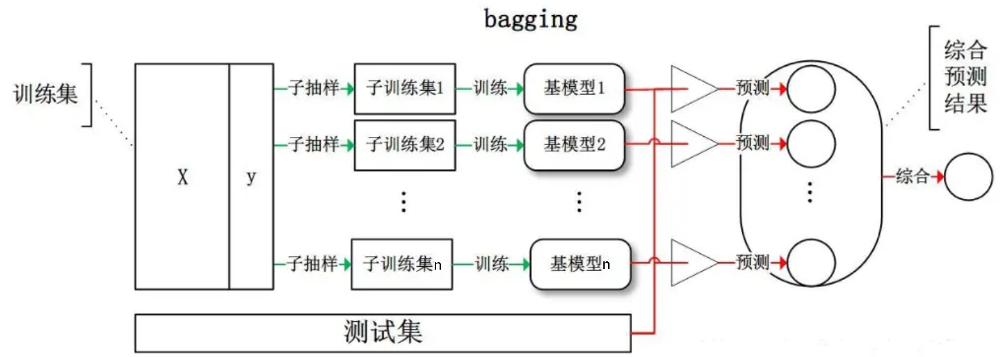
【Bagging】
Bagging 装袋法,是集成学习的经典算法之一,其本质是引入样本扰动,通过增加样本随机性,以降低方差
Bagging 基于自助采样法(Bootstrap Sampling),即:给定包含 $n$ 个样本的数据集 $D$,每轮有放回的随机选出一个样本放入采样集 $D’$ 中,经过 $n$ 次随机采样后,可以得到包含 $n$ 个样本的采样集 $D’$,有的样本在采样集中多次出现,有的样本在采样集中从未出现
通过自主采样法,初始数据集 $D$ 中约有 $36.8\%$ 的样本从未出现过采样数据集 $D’$ 中
这样一来,可以采样出 $T$ 个含 $n$ 个训练样本的采样集,然后基于每个采样集训练出一个基学习器,最后再将这些基学习器进行结合
对于分类任务,Bagging 常采用相对多数投票法作为结合策略,对于回归任务,则采用简单平均法作为结合策略
关于自助采样法,详见:机器学习的模型选择
【模型平均】
Bagging 是通过结合几个基学习器来降低泛化误差的技术,主要想法是分别训练几个不同的模型,然后让所有模型表决测试样例的输出,这种思想被称为模型平均(Model Averaging)
模型平均奏效的原因是不同的学习器通常不会在测试集上产生完全相同的误差,其是一种减少泛化误差的非常强大可靠的方法
此外,从偏差-方差分解的角度来看,Bagging 主要关注于降低方差,因此它在不剪枝的决策树、神经网络等容易受到样本扰动的学习器上效果更明显
【包外估计】
使用 Bagging 来产生训练数据集有一个好处是,没有必要再使用交叉验证或使用一个独立的测试集来获取误差的无偏估计
这是因为每个基学习器只使用了训练集中约 $63.2\%$ 的样本,剩下的 $36.8\%$ 的样本可用作验证集来对泛化性能进行评估,这种评估方式被称为包外估计(Out-of-bag Estimate)
记 $D_t$ 为基学习器 $f_t(\mathbf{x})$ 所实际使用的训练样本集,令 $H^{\text{oob}}(\mathbf{x})$ 为样本 $\mathbf{x}$ 的包外预测,即仅考虑未使用 $\mathbf{x}$ 训练的基学习器在 $\mathbf{x}$ 上的预测,有:
则 Bagging 泛化误差的包外估计为:
包外估计 $\varepsilon^{\text{oob}}$ 是对泛化误差的一个无偏估计,其结果近似于需要大量计算的 $k$ 折交叉验证
此外,包外样本还有诸多用途,例如:当基学习器是决策树时,可使用包外样本来辅助剪枝,或用于估价决策树中各结点的后验概率以辅助对训练样本结点的处理;当基学习器是神经网络时,可使用包外样本来辅助提前停止,以减小过拟合
【随机森林】
随机森林(Random Forest,RF)是通过 Bagging 将决策树作为基学习器的集成学习算法

随机森林中的随机,是指两个随机性,一个是对训练集采用 Bagging 生成采样训练集来训练基决策树,另一个是在决策树的基础上引入了随机特征选择
具体来说,传统决策树在选择划分特征时,是在当前结点的特征集合中选择一个最优特征
而随机森林是对于基决策树的每个结点,从该结点的 $d$ 个特征中随机选择一个包含 $k$ 个特征的子集,然后再从这个子集中选择一个最优特征用于划分
其中,$k$ 控制了随机性的引入程度,若 $k=d$,则基决策树的构建与传统决策树相同,若 $k=1$,则是随机选择一个特征进行划分,一般情况下,推荐 $k=\log_2 d$
【sklearn 实现】
Bagging
在 sklearn 中看,Bagging 有两种,一种是用于回归的 BaggingRegressor(),另一种是用于分类的 BaggingClassifier()
1 | from sklearn.svm import SVC |
随机森林
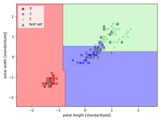
以 sklearn 中的鸢尾花数据集为例,选取其后两个特征来实现随机森林
1 | import pandas as pd |